使用 RegVelo 进行 RNA velocity 和调控扰动分析#
RegVelo 是一个 gene-regulatory-informed RNA velocity 模型,目标是在单细胞层面同时建模转录调控和 RNA splicing dynamics。传统 RNA velocity 方法通常根据 unspliced/spliced RNA 的变化推断细胞状态转移,但对 TF-regulon、GRN 先验和调控扰动的利用有限;而单独的 GRN 推断又往往缺少表达动态和细胞时间的信息。RegVelo 将这两类信息放到同一个生成式动力学框架中,用先验 GRN 约束转录率,并通过耦合的 ODE 系统推断 velocity、latent time 以及调控扰动后的 vector field。

从算法流程看,RegVelo 的输入包括包含 spliced/unspliced moment layer 的 AnnData、与基因空间对齐的 prior GRN,以及 TF/regulator 列表。模型会学习基因调控网络约束下的 splicing kinetics,并把结果导出为 velocity layer、latent time、gene-level kinetic parameters 和可用于下游 CellRank 的 velocity field。进一步地,训练好的 RegVelo 模型可以进行 in silico TF regulon blockade:通过移除某个 TF 的 downstream regulatory effects 生成扰动后的 velocity field,再结合 CellRank 比较原始和扰动条件下的 fate probabilities,从而连接局部调控变化与长期细胞命运偏移。
在 OmicVerse 中,我们保留了 RegVelo 的上游模型语义,同时让结果回到 adata 来保持与其他方法的统一。本教程使用 adata-first 的 ov.single.velocity(..., method="regvelo") 完成 velocity 推断,并用 ov.single.cellrank_fate() 与 ov.pl.cell_fate() 进行 CellRank fate analysis 和可视化。示例数据沿用 RegVelo 官方 zebrafish neural crest 教程,但流程被整理为 OmicVerse 风格:显式读取示例数据、准备 RegVelo 输入、推断 velocity、绘制 streamplot、连接 CellRank fate analysis,并进行 TF 扰动模拟。
import numpy as np
import warnings
warnings.filterwarnings("ignore", category=FutureWarning)

import omicverse as ov
import regvelo as rgv

ov.plot_set(font_path="Arial")

%reload_ext autoreload
%autoreload 2
🔬 Starting plot initialization...
Using already downloaded Arial font from: /var/folders/rv/3jnfbs0d6r7d0c5bfj7ft5k00000gn/T/omicverse_arial.ttf
Registered as: Arial
🧬 Detecting GPU devices…
✅ Apple Silicon MPS detected
    • [MPS] Apple Silicon GPU - Metal Performance Shaders available

   ____            _     _    __
  / __ \____ ___  (_)___| |  / /__  _____________
 / / / / __ `__ \/ / ___/ | / / _ \/ ___/ ___/ _ \
/ /_/ / / / / / / / /__ | |/ /  __/ /  (__  )  __/
\____/_/ /_/ /_/_/\___/ |___/\___/_/  /____/\___/

🔖 Version: 2.1.3rc1   📚 Tutorials: https://omicverse.readthedocs.io/
✅ plot_set complete.
读取 RegVelo 官方示例数据并用 OmicVerse 预处理#
这里仍然沿用 RegVelo 上游 zebrafish neural crest 教程的数据,但把“示例数据读取”和“RegVelo 预处理”分开:数据加载直接使用上游 regvelo.datasets,OmicVerse 只负责拿到 adata 后的 neighbor/moment、RegVelo gene preprocessing 和 GRN 对齐。
这种写法避免在 OmicVerse 中增加额外的数据下载入口,也更接近真实项目:你可以把 rgv.datasets.zebrafish_nc() 换成自己的 AnnData,把 rgv.datasets.zebrafish_grn() 换成自己的 prior GRN;后续预处理、velocity 计算和可视化仍然走同一套 OmicVerse 流程。
adata = rgv.datasets.zebrafish_nc()
prior_net = rgv.datasets.zebrafish_grn()

velo_prep = ov.single.Velo(adata)
prior_grn, regulators = velo_prep.prepare_regvelo(
    prior_net,
    n_neighbors=30,
    n_pcs=50,
    moment_backend="scvelo",
    prior_orientation="regulator_by_target",
)
adata = velo_prep.adata

print(adata)
print("Available layers:", list(adata.layers.keys())[:10])
print("Prior GRN shape:", prior_grn.shape)
print("TFs retained:", len(regulators))
In Velo module, you should keep all genes' expression not normalized.
🖥️ Using Scanpy CPU to calculate neighbors...

🔍 K-Nearest Neighbors Graph Construction:
   Mode: cpu
   Neighbors: 30
   Method: umap
   Metric: euclidean
   PCs used: 50
   🔍 Computing neighbor distances...
   🔍 Computing connectivity matrix...
   💡 Using UMAP-style connectivity
✓ Graph is fully connected

✅ KNN Graph Construction Completed Successfully!
   ✓ Processed: 697 cells with 30 neighbors each
   ✓ Results added to AnnData object:
     • 'neighbors': Neighbors metadata (adata.uns)
     • 'distances': Distance matrix (adata.obsp)
     • 'connectivities': Connectivity matrix (adata.obsp)

╭─ SUMMARY: neighbors ───────────────────────────────────────────────╮
│  Duration: 2.1564s                                                 │
│  Shape:    697 x 8,012 (Unchanged)                                 │
│                                                                    │
│  CHANGES DETECTED                                                  │
│  ────────────────                                                  │
│  ● UNS    │ ✚ REFERENCE_MANU                                       │
│           │ ✚ _ov_provenance                                       │
│           │ ✚ neighbors                                            │
│           │ └─ params: {'n_neighbors': 30, 'method': 'umap', 'random_s...│
│                                                                    │
│  ● OBSP   │ ✚ connectivities (sparse matrix, 697x697)              │
│           │ ✚ distances (sparse matrix, 697x697)                   │
│                                                                    │
╰────────────────────────────────────────────────────────────────────╯
computing moments based on connectivities
finished (0:00:00) --> added
    'Ms' and 'Mu', moments of un/spliced abundances (adata.layers)
computing velocities
    finished (0:00:00) --> added
    'velocity', velocity vectors for each individual cell (adata.layers)
AnnData object with n_obs × n_vars = 697 × 1008
    obs: 'initial_size_unspliced', 'initial_size_spliced', 'initial_size', 'n_counts', 'cell_type', 'stage'
    var: 'Accession', 'Chromosome', 'End', 'Start', 'Strand', 'gene_count_corr', 'is_tf', 'velocity_gamma', 'velocity_qreg_ratio', 'velocity_r2', 'velocity_genes'
    uns: 'cell_type_colors', 'neighbors', 'REFERENCE_MANU', '_ov_provenance', 'history_log', 'velocity_params', 'regulators', 'targets', 'skeleton', 'network', 'regvelo_prepare', 'regvelo_regulators'
    obsm: 'X_pca', 'X_umap'
    layers: 'ambiguous', 'matrix', 'spliced', 'unspliced', 'Ms', 'Mu', 'velocity'
    obsp: 'distances', 'connectivities'
Available layers: ['ambiguous', 'matrix', 'spliced', 'unspliced', 'Ms', 'Mu', 'velocity']
Prior GRN shape: (1008, 1008)
TFs retained: 81
使用 OmicVerse 准备好的 prior GRN#
Velo.prepare_regvelo() 会把对齐后的 prior network 写入 adata.uns["skeleton"],并把保留下来的 regulator 列表写入 adata.uns["regvelo_regulators"]。RegVelo zebrafish helper 读取的上游 prior 是 regulator-by-target 方向;OmicVerse 会保存对齐后的 adata.uns["skeleton"],并由 ov.single.velocity(..., method="regvelo") 处理 REGVELOVI 需要的方向。
prior_grn = adata.uns["skeleton"]
regulators = adata.uns["regvelo_regulators"]

print("Prior GRN shape:", prior_grn.shape)
print("Regulators:", len(regulators))
Prior GRN shape: (1008, 1008)
Regulators: 81
通过 ov.single.velocity 运行 RegVelo#
RegVelo 分支现在可以作为 adata-first velocity 流程使用:训练上游模型,把 layers["velocity"] 导出到 layers["velo_regvelo"],可选地直接构建 velocity graph、投影到 UMAP,在 adata.uns["regvelo"] 记录参数,并保留模型路径供后续扰动分析使用。
adata = ov.single.velocity(
    adata,
    method="regvelo",
    prior_grn=prior_grn,
    regulators=regulators,
    model_save_path="result/regvelo_zebrafish",
    model_overwrite=True,
    velocity_key="velo_regvelo",
    spliced_layer="Ms",
    unspliced_layer="Mu",
    n_samples=30,
    regvelo_kwargs={
        "soft_constraint": False,
    },
    train_kwargs={
        "max_epochs": 50,  # 测试中使用较小 epochs,请根据真实数据调整
    },
    compute_velocity_graph=True,
    compute_velocity_embedding=True,
    basis="umap",
    graph_kwargs={
        "xkey": "Ms",
    },
)
In Velo module, you should keep all genes' expression not normalized.
computing velocity graph (using 1/12 cores)
finished (0:00:00) --> added
    'velo_regvelo_graph', sparse matrix with cosine correlations (adata.uns)
computing velocity embedding
    finished (0:00:00) --> added
    'velo_regvelo_umap', embedded velocity vectors (adata.obsm)
可视化 RegVelo vector field#
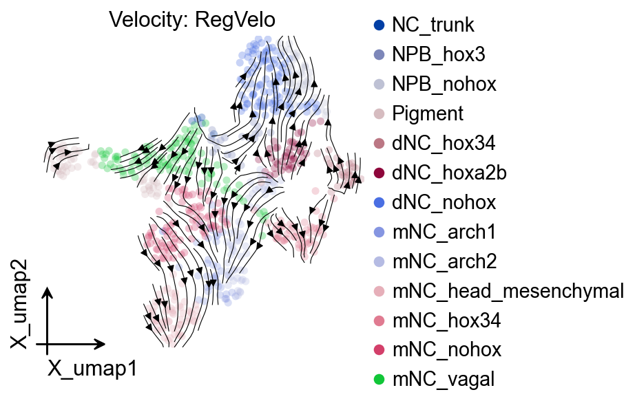
这里直接使用 OmicVerse 绘图函数从 adata 读取结果。ov.pl.embedding() 绘制细胞嵌入,ov.pl.add_streamplot() 叠加 adata.obsm["velo_regvelo_umap"] 中的 velocity field。
adata.uns["regvelo"]
{'spliced_layer': 'Ms',
 'unspliced_layer': 'Mu',
 'n_samples': 30,
 'batch_size': 697,
 'velocity_key': 'velo_regvelo',
 'n_regulators': 81,
 'model_load_path': None,
 'model_save_path': 'result/regvelo_zebrafish',
 'model_overwrite': True,
 'reuse_regvelo_output': False,
 'reused_regvelo_output': False}
fig = ov.plt.figure(figsize=(4, 4))
ax = ov.plt.subplot(1, 1, 1)

ov.pl.embedding(
    adata,
    basis="X_umap",
    color="cell_type",
    ax=ax,
    show=False,
    size=100,
    alpha=0.3,
)
ov.pl.add_streamplot(
    adata,
    basis="X_umap",
    velocity_key="velo_regvelo_umap",
    ax=ax,
)
ov.plt.title("Velocity: RegVelo")
Text(0.5, 1.0, 'Velocity: RegVelo')
检查 latent time 和 regulon size#
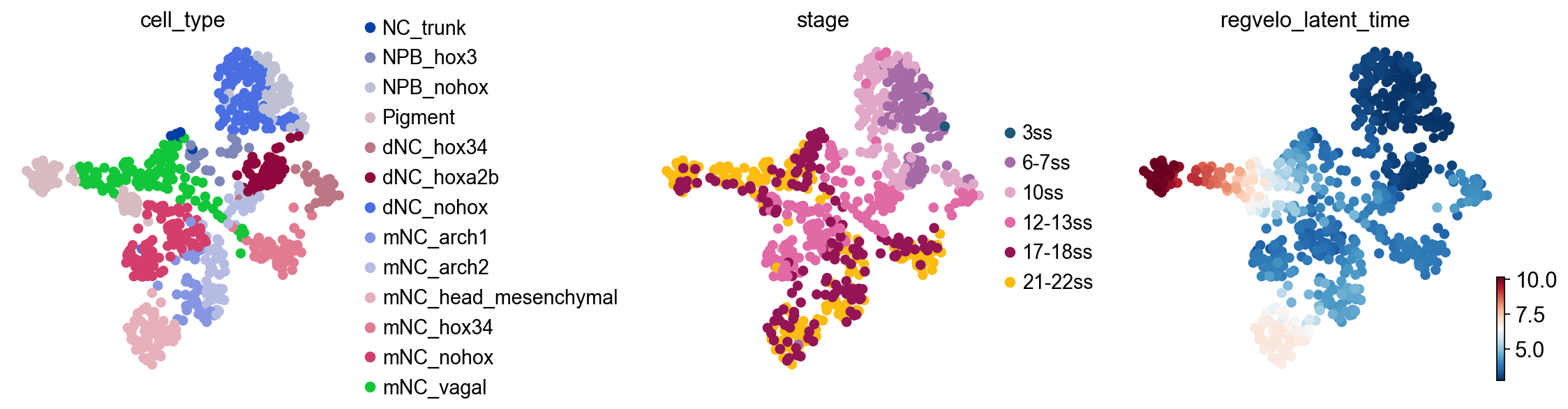
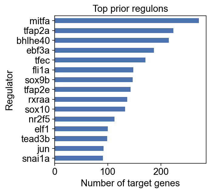
检查 latent time 和 GRN 结构。不同 RegVelo 版本导出的对象可能略有差异,因此这里先检查是否存在 fit_t,再绘制 latent time;同时从 adata.uns["skeleton"] 汇总 prior regulon 大小。
fit_t = np.asarray(adata.layers["fit_t"])
adata.obs["regvelo_latent_time"] = fit_t.mean(axis=1)

ov.pl.embedding(
    adata,
    basis="X_umap",
    color=["cell_type", "stage", "regvelo_latent_time"],
    ncols=3,
    frameon=False,
    show=False,
)
[<Axes: title={'center': 'cell_type'}, xlabel='X_umap1', ylabel='X_umap2'>,
 <Axes: title={'center': 'stage'}, xlabel='X_umap1', ylabel='X_umap2'>,
 <Axes: title={'center': 'regvelo_latent_time'}, xlabel='X_umap1', ylabel='X_umap2'>]
regulon_size = (prior_grn != 0).sum(axis=1).sort_values(ascending=False).head(15)
ax = regulon_size.sort_values().plot.barh(figsize=(4, 4), color="#4c72b0")
ax.set_xlabel("Number of target genes")
ax.set_ylabel("Regulator")
ax.set_title("Top prior regulons")
Text(0.5, 1.0, 'Top prior regulons')
基于 RegVelo velocity 的 CellRank fate analysis#
ov.single.cellrank_fate() 会从 adata.layers["velo_regvelo"] 构建 CellRank velocity kernel,可选混入 connectivity kernel,计算 GPCCA macrostates,并把 estimator/kernel 保存到 adata.uns["velocity_cellrank"]。后续可直接用 ov.pl.cell_fate(adata, ...) 可视化,不需要依赖 wrapper 对象。
terminal_states = ["mNC_head_mesenchymal", "mNC_hox34", "Pigment"]
terminal_states = [state for state in terminal_states if state in set(adata.obs["cell_type"])]
if not terminal_states:
    raise ValueError("None of the tutorial terminal states were found in adata.obs['cell_type'].")

estimator = ov.single.cellrank_fate(
    adata,
    velocity_key="velo_regvelo",
    xkey="Ms",
    cluster_key="cell_type",
    terminal_states=terminal_states,
    n_states=7,
    n_cells=30,
    connectivity_weight=0.2,
    compute_fate_probabilities=True,
    plot=False,
)
In Velo module, you should keep all genes' expression not normalized.
WARNING: Unable to import `petsc4py` or `slepc4py`. Using `method='brandts'`
WARNING: For `method='brandts'`, dense matrix is required. Densifying
WARNING: Unable to import petsc4py. For installation, please refer to: https://petsc4py.readthedocs.io/en/stable/install.html.
Defaulting to `'gmres'` solver.
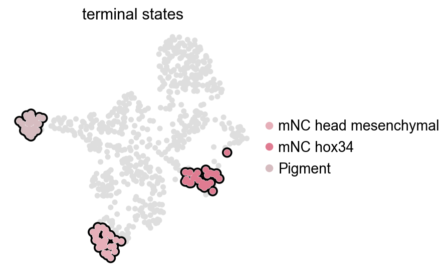
ov.pl.cell_fate() 会复用 adata.uns["velocity_cellrank"]["estimator"] 中保存的 CellRank 结果。它只负责可视化,不会重新计算 terminal states。
ov.pl.cell_fate(adata, which="terminal", basis="umap")
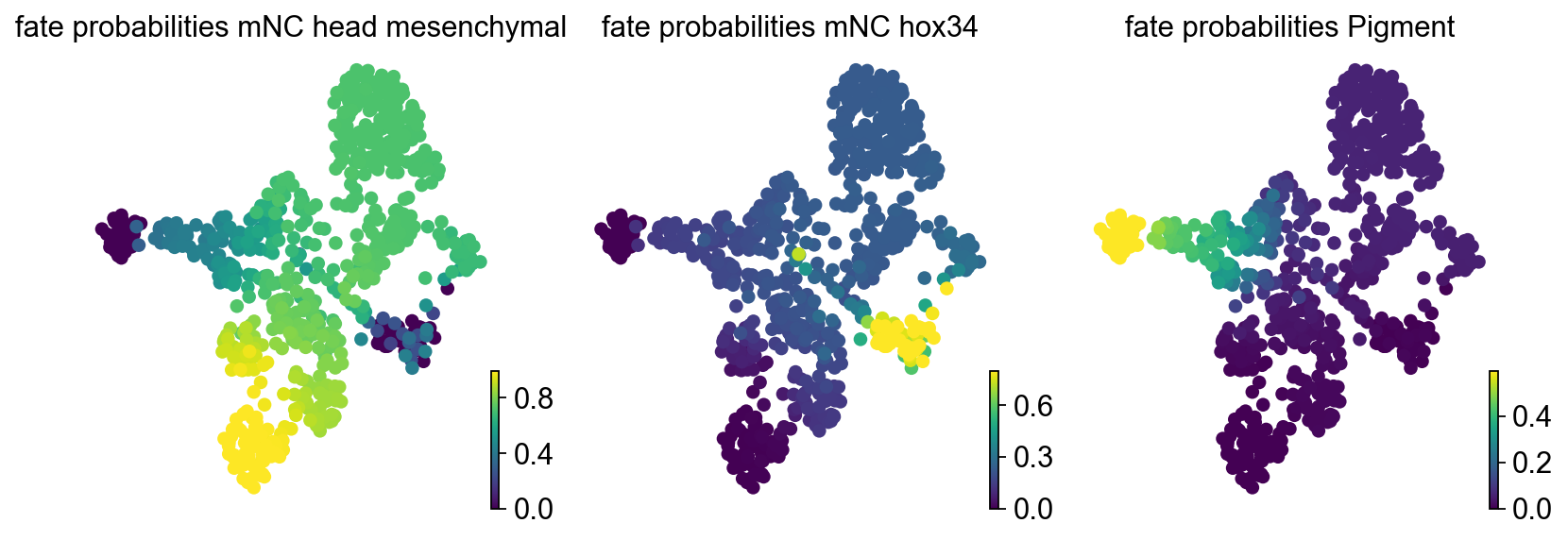
fate probabilities 与 commitment score#
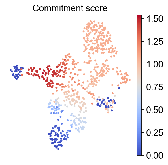
除了 terminal state 点图,RegVelo 官方扰动教程还会查看 CellRank 的 fate probabilities 和 commitment score。commitment_score 基于 fate probability distribution 的 entropy;数值越低通常表示细胞命运越 committed。
estimator.plot_fate_probabilities(
    same_plot=False,
    basis="umap",
)
rgv.pl.commitment_score(
    adata=adata,
    lineage_key="lineages_fwd",
    frameon=False,
    s=40,
    cmap="coolwarm",
    title="Commitment score",
)
RegVelo 原生 TF regulon 阻断模拟#
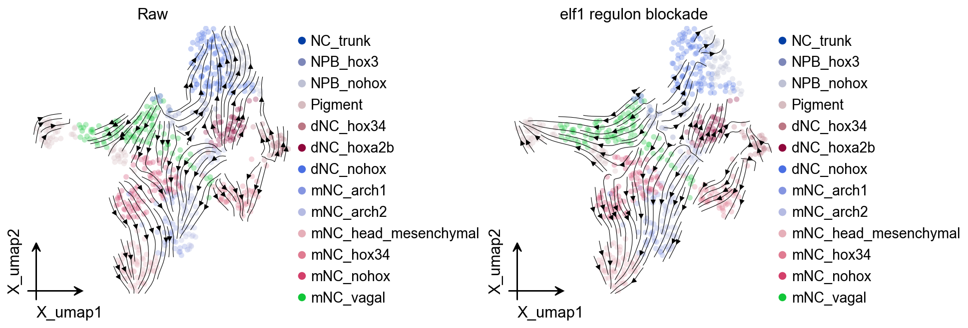
复现仓库会使用保存的 RegVelo model 做 TF perturbation 和 regulatory screening。由于 ov.single.velocity(method="regvelo") 已经把模型路径记录到 adata.uns["regvelo_model_path"],这里临时构建一个轻量 Velo helper 来继续调用 RegVelo 原生扰动 API。
velo_helper = ov.single.Velo(adata)
elf1_perturbed_adata, elf1_perturbed_model = velo_helper.regvelo_perturb(
    "elf1",
    model="result/regvelo_zebrafish",
    cutoff=0.001,
    batch_size=adata.n_obs,
)

print(elf1_perturbed_adata)
In Velo module, you should keep all genes' expression not normalized.
INFO     File result/regvelo_zebrafish/model.pt already downloaded
AnnData object with n_obs × n_vars = 697 × 1008
    obs: 'initial_size_unspliced', 'initial_size_spliced', 'initial_size', 'n_counts', 'cell_type', 'stage', 'velo_regvelo_self_transition', 'regvelo_latent_time', 'macrostates_fwd', 'term_states_fwd', 'term_states_fwd_probs', 'commitment_score'
    var: 'Accession', 'Chromosome', 'End', 'Start', 'Strand', 'gene_count_corr', 'is_tf', 'velocity_gamma', 'velocity_qreg_ratio', 'velocity_r2', 'velocity_genes', 'fit_beta', 'fit_gamma', 'fit_scaling', 'velo_regvelo_genes'
    uns: 'cell_type_colors', 'neighbors', 'REFERENCE_MANU', '_ov_provenance', 'history_log', 'velocity_params', 'regulators', 'targets', 'skeleton', 'network', 'regvelo_prepare', 'regvelo_regulators', '_scvi_uuid', '_scvi_manager_uuid', 'regvelo_model_path', 'regvelo', 'velo_regvelo_graph', 'velo_regvelo_graph_neg', 'velo_regvelo_params', 'stage_colors_rgba', 'stage_colors', 'schur_matrix_fwd', 'eigendecomposition_fwd', 'macrostates_fwd_colors', 'coarse_fwd', 'term_states_fwd_colors', 'velocity_cellrank'
    obsm: 'X_pca', 'X_umap', 'velo_regvelo_umap', 'schur_vectors_fwd', 'macrostates_fwd_memberships', 'term_states_fwd_memberships', 'lineages_fwd'
    layers: 'ambiguous', 'matrix', 'spliced', 'unspliced', 'Ms', 'Mu', 'velocity', 'latent_time_velovi', 'fit_t', 'velo_regvelo', 'latent_time_regvelo'
    obsp: 'distances', 'connectivities'
fig, axes = ov.plt.subplots(1, 2, figsize=(12, 4), constrained_layout=True)

ov.pl.embedding(
    adata,
    basis="X_umap",
    color="cell_type",
    ax=axes[0],
    show=False,
    size=100,
    alpha=0.3,
)
ov.pl.add_streamplot(
    adata,
    basis="X_umap",
    velocity_key="velo_regvelo_umap",
    ax=axes[0],
)
axes[0].set_title("Raw")

elf1_perturbed_velo = ov.single.Velo(elf1_perturbed_adata)
elf1_perturbed_velo.velocity_graph(vkey="velocity", xkey="Ms", n_jobs=8)
elf1_perturbed_velo.velocity_embedding(basis="umap", vkey="velocity")

ov.pl.embedding(
    elf1_perturbed_adata,
    basis="X_umap",
    color="cell_type",
    ax=axes[1],
    show=False,
    size=100,
    alpha=0.3,
)
ov.pl.add_streamplot(
    elf1_perturbed_adata,
    basis="X_umap",
    velocity_key="velocity_umap",
    ax=axes[1],
)
axes[1].set_title("elf1 regulon blockade")

ov.plt.show()
In Velo module, you should keep all genes' expression not normalized.
computing velocity graph (using 8/12 cores)
finished (0:00:06) --> added
    'velocity_graph', sparse matrix with cosine correlations (adata.uns)
computing velocity embedding
    finished (0:00:00) --> added
    'velocity_umap', embedded velocity vectors (adata.obsm)
量化 TF blockade 的影响#
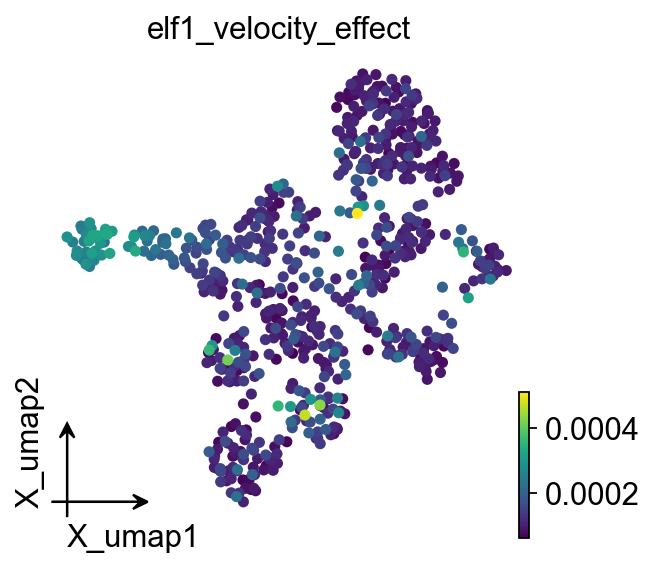
除了 streamplot 可视化,还可以进一步比较扰动前后的 velocity field 和 CellRank fate probabilities。 这里给出两个互补指标:
局部效应:每个 cell 的 velocity cosine dissimilarity,数值越大表示扰动后方向改变越明显。
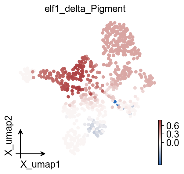
命运效应:重新用扰动后的 velocity field 计算 CellRank fate probabilities,再比较 terminal fate probability 的增加或降低。
ov.single.velocity_effect(
    adata,
    elf1_perturbed_adata,
    baseline_velocity_key="velo_regvelo",
    perturbed_velocity_key="velocity",
    target="elf1",
)

velocity_effect_summary = (
    adata.obs.groupby("cell_type", observed=True)["elf1_velocity_effect"]
    .agg(["mean", "median", "max"])
    .sort_values("mean", ascending=False)
)
velocity_effect_summary
In Velo module, you should keep all genes' expression not normalized.
                          mean    median       max
cell_type
Pigment               0.000225  0.000252  0.000334
NPB_hox3              0.000189  0.000152  0.000511
NC_trunk              0.000176  0.000148  0.000277
mNC_vagal             0.000152  0.000144  0.000268
mNC_arch1             0.000149  0.000132  0.000468
dNC_hox34             0.000136  0.000111  0.000351
mNC_arch2             0.000130  0.000114  0.000432
mNC_nohox             0.000121  0.000106  0.000414
mNC_hox34             0.000120  0.000109  0.000314
mNC_head_mesenchymal  0.000109  0.000097  0.000223
dNC_nohox             0.000107  0.000099  0.000226
dNC_hoxa2b            0.000105  0.000101  0.000165
NPB_nohox             0.000100  0.000091  0.000203
ov.pl.embedding(
    adata,
    basis="X_umap",
    color="elf1_velocity_effect",
    cmap="viridis",
    size=100,
)
elf1_estimator = ov.single.cellrank_fate(
    elf1_perturbed_adata,
    velocity_key="velocity",
    xkey="Ms",
    cluster_key="cell_type",
    terminal_states=terminal_states,
    n_states=7,
    n_cells=30,
    connectivity_weight=0.2,
    compute_fate_probabilities=True,
    plot=False,
)
In Velo module, you should keep all genes' expression not normalized.
WARNING: Unable to import `petsc4py` or `slepc4py`. Using `method='brandts'`
WARNING: For `method='brandts'`, dense matrix is required. Densifying
import pandas as pd

def _lineage_to_df(adata_obj, key="lineages_fwd"):
    lineages = adata_obj.obsm[key]
    values = np.asarray(lineages)
    names = getattr(lineages, "names", None)
    if names is None:
        names = [f"lineage_{i}" for i in range(values.shape[1])]
    return pd.DataFrame(values, index=adata_obj.obs_names, columns=list(names))

baseline_fate = _lineage_to_df(adata)
elf1_fate = _lineage_to_df(elf1_perturbed_adata)
common_fates = baseline_fate.columns.intersection(elf1_fate.columns)

elf1_fate_delta = elf1_fate[common_fates] - baseline_fate[common_fates]
elf1_fate_delta.columns = [f"elf1_delta_{state}" for state in common_fates]
adata.obs = adata.obs.join(elf1_fate_delta)

elf1_fate_delta_summary = elf1_fate_delta.groupby(adata.obs["cell_type"], observed=True).mean()
elf1_fate_delta_summary
                      elf1_delta_mNC_head_mesenchymal  elf1_delta_mNC_hox34  \
cell_type
NC_trunk                                    -0.459529             -0.127518
NPB_hox3                                    -0.367804             -0.070306
NPB_nohox                                   -0.298640             -0.044843
Pigment                                     -0.203943             -0.072228
dNC_hox34                                   -0.263292             -0.030998
dNC_hoxa2b                                  -0.283801             -0.043709
dNC_nohox                                   -0.296808             -0.044384
mNC_arch1                                    0.074196             -0.105023
mNC_arch2                                    0.026702             -0.107880
mNC_head_mesenchymal                         0.003305             -0.003480
mNC_hox34                                    0.034400             -0.064902
mNC_nohox                                   -0.082420             -0.098148
mNC_vagal                                   -0.455308             -0.137573

                      elf1_delta_Pigment
cell_type
NC_trunk                        0.587044
NPB_hox3                        0.438102
NPB_nohox                       0.343470
Pigment                         0.276171
dNC_hox34                       0.294278
dNC_hoxa2b                      0.327496
dNC_nohox                       0.341179
mNC_arch1                       0.030827
mNC_arch2                       0.081175
mNC_head_mesenchymal            0.000176
mNC_hox34                       0.030502
mNC_nohox                       0.180568
mNC_vagal                       0.592879
ov.pl.embedding(
    adata,
    basis="X_umap",
    color="elf1_delta_Pigment",
    cmap="vlag",
    vcenter=0,
    size=100,
)
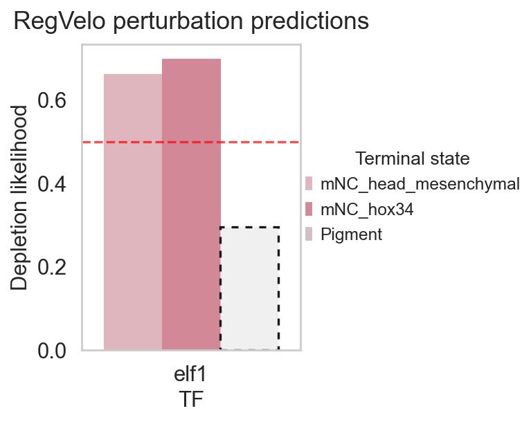
RegVelo 也提供原生的 fate perturbation 统计函数,用于把扰动后的 fate probability depletion/enrichment 汇总成表。这里通过 ov.single.cell_fate_perturbation() 统一调用,OmicVerse 会在内部兼容不同 RegVelo 版本中的 metrics / mt 路径。
elf1_fate_stats = ov.single.cell_fate_perturbation(
    adata,
    perturbed={"elf1": elf1_perturbed_adata},
    terminal_states=terminal_states,
    score_method="likelihood",
)
elf1_fate_stats
In Velo module, you should keep all genes' expression not normalized.
   Depletion likelihood       p-value  FDR adjusted p-value  \
0              0.661134  1.041763e-25          1.562645e-25
1              0.698439  5.703815e-38          1.711145e-37
2              0.295141  1.000000e+00          1.000000e+00

         Terminal state    TF
0  mNC_head_mesenchymal  elf1
1             mNC_hox34  elf1
2               Pigment  elf1
rgv.pl.cellfate_perturbation(
    adata=adata,
    df=elf1_fate_stats,
    color_label="cell_type",
    figsize=(5, 4),
)
Single-cell perturbation effect#
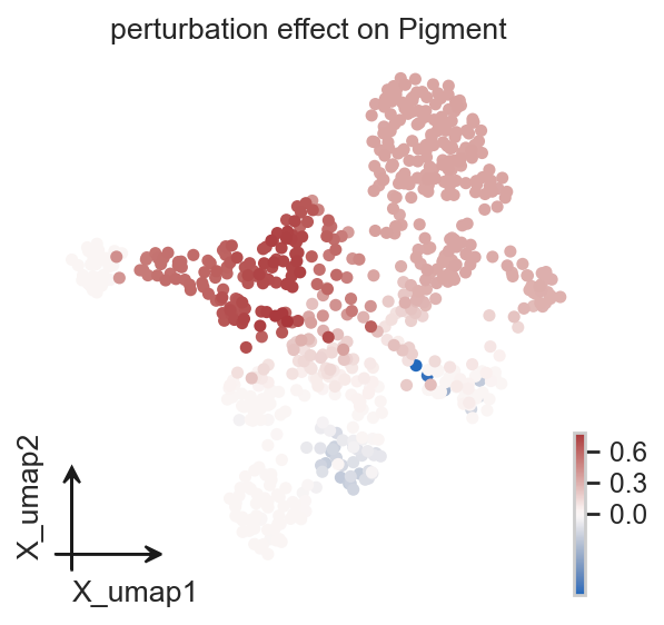
ov.single.perturbation_effect() 用于把扰动前后的 fate probability 差异写回 adata.obs。负值表示该 cell 朝某个 terminal fate 的 probability 降低,正值表示升高。
adata = ov.single.perturbation_effect(
    adata,
    elf1_perturbed_adata,
    terminal_states=terminal_states,
)

effect_cols = [col for col in adata.obs.columns if col.startswith("perturbation effect on ")]
print(effect_cols)
In Velo module, you should keep all genes' expression not normalized.
['perturbation effect on mNC_head_mesenchymal', 'perturbation effect on mNC_hox34', 'perturbation effect on Pigment']
effect_key = "perturbation effect on Pigment"
ov.pl.embedding(
    adata,
    basis="X_umap",
    color=effect_key,
    cmap="vlag",
    vcenter=0,
    size=100,
)
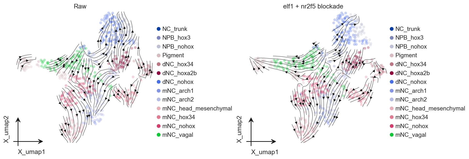
多个 TF 同时 blockade#
regvelo_perturb() 的 tf 参数也可以传入多个 TF。多 TF 组合扰动通常用于探索协同调控,但建议先确认这些 TF 都在当前模型保留的 regulator 列表中。
multi_tfs = ["elf1", "nr2f5"]
multi_tfs = [tf for tf in multi_tfs if tf in adata.var_names]

multi_perturbed_adata, multi_perturbed_model = ov.single.Velo(adata).regvelo_perturb(
    multi_tfs,
    model="result/regvelo_zebrafish",
    cutoff=0.001,
    batch_size=adata.n_obs,
)

multi_perturbed_velo = ov.single.Velo(multi_perturbed_adata)
multi_perturbed_velo.velocity_graph(vkey="velocity", xkey="Ms", n_jobs=8)
multi_perturbed_velo.velocity_embedding(basis="umap", vkey="velocity")
In Velo module, you should keep all genes' expression not normalized.
INFO     File result/regvelo_zebrafish/model.pt already downloaded
In Velo module, you should keep all genes' expression not normalized.
computing velocity graph (using 8/12 cores)
finished (0:00:01) --> added
    'velocity_graph', sparse matrix with cosine correlations (adata.uns)
computing velocity embedding
    finished (0:00:00) --> added
    'velocity_umap', embedded velocity vectors (adata.obsm)
fig, axes = ov.plt.subplots(1, 2, figsize=(12, 4), constrained_layout=True)

ov.pl.embedding(
    adata,
    basis="X_umap",
    color="cell_type",
    ax=axes[0],
    show=False,
    size=100,
    alpha=0.3,
)
ov.pl.add_streamplot(
    adata,
    basis="X_umap",
    velocity_key="velo_regvelo_umap",
    ax=axes[0],
)
axes[0].set_title("Raw")

ov.pl.embedding(
    multi_perturbed_adata,
    basis="X_umap",
    color="cell_type",
    ax=axes[1],
    show=False,
    size=100,
    alpha=0.3,
)
ov.pl.add_streamplot(
    multi_perturbed_adata,
    basis="X_umap",
    velocity_key="velocity_umap",
    ax=axes[1],
)
axes[1].set_title("elf1 + nr2f5 blockade")

ov.plt.show()