带参考 scRNA-seq 的空间反卷积

这个教程展示了如何使用参考 scRNA-seq 数据进行空间反卷积。

import squidpy as sq
import omicverse as ov
# print(f"omicverse version: {ov.__version__}")
import scanpy as sc

🔬 Starting plot initialization...
Using already downloaded Arial font from: /tmp/omicverse_arial.ttf
Registered as: Arial
🧬 Detecting GPU devices…
✅ NVIDIA CUDA GPUs detected: 1
    • [CUDA 0] NVIDIA H100 80GB HBM3
      Memory: 79.1 GB | Compute: 9.0

   ____            _     _    __                  
  / __ \____ ___  (_)___| |  / /__  _____________ 
 / / / / __ `__ \/ / ___/ | / / _ \/ ___/ ___/ _ \ 
/ /_/ / / / / / / / /__ | |/ /  __/ /  (__  )  __/ 
\____/_/ /_/ /_/_/\___/ |___/\___/_/  /____/\___/                                              

🔖 Version: 1.7.8rc1   📚 Tutorials: https://omicverse.readthedocs.io/
✅ plot_set complete.

第1步：准备 scRNA-seq 参考 (1 分钟)

目的：加载和标准化单细胞参考数据。

# 加载参考
adata_sc = sc.read_h5ad('data/reference.h5ad')

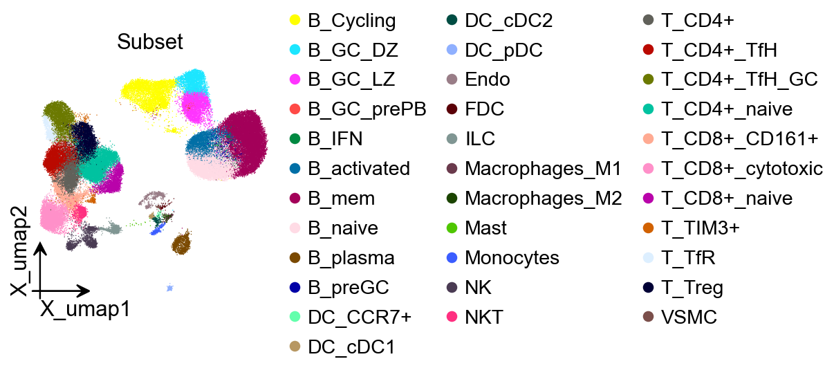
<Axes: title={'center': 'Subset'}, xlabel='X_umap1', ylabel='X_umap2'>

步骤 2: Prepare 空间转录组学 (1 min)Purpose: 加载 10x Visium (Space Ranger outputs) 或 similar 到 obtain a coordinate-aware spatial AnnData (adata_sp).- Inputs: Visium 计数 矩阵 和 spatial coordinates (从 该 spatial 文件夹)- Outputs: AnnData object (adata_sp) 使用 点位 coordinates 和 计数- Key points: - Ensure maximal 基因 overlap 使用 该 scRNA-seq 参考; map 基因 IDs 如果 necessary. - 对于 multiple samples, keep batch 标签 explicit 到 support merging 和 可视化.

adata_sp = sc.datasets.visium_sge(sample_id="V1_Human_Lymph_Node")adata_sp.obs['sample'] = list(adata_sp.uns['spatial'].keys())[0]adata_sp.var_names_make_unique()

reading /scratch/users/steorra/analysis/omic_test/data/V1_Human_Lymph_Node/filtered_feature_bc_matrix.h5
 (0:00:00)

步骤 3: Tangram 解卷积 (15–30 min)Tangram maps scRNA-seq 表达 into spatial coordinates 到 infer 细胞类型 分布 和 proportions. We use omicverse.space.Deconvolution 对于 a consistent interface.

decov_obj=ov.space.Deconvolution(    adata_sc=adata_sc,    adata_sp=adata_sp)

步骤 3.1 Tangram preprocessingPurpose: prepare scRNA-seq 和 spatial 数据 使用 necessary 筛选/transformations 到 enable 稳健 fitting (prefer raw 计数).

decov_obj.preprocess_sc(    mode='shiftlog|pearson',n_HVGs=3000,target_sum=1e4,)decov_obj.preprocess_sp(    mode='pearsonr',n_svgs=3000,target_sum=1e4,)

🔍 [2025-09-20 03:25:56] Running preprocessing in 'cpu' mode...
Begin robust gene identification
    After filtration, 10237/10237 genes are kept.
    Among 10237 genes, 9838 genes are robust.
✅ Robust gene identification completed successfully.
Begin size normalization: shiftlog and HVGs selection pearson

🔍 Count Normalization:
   Target sum: 10000.0
   Exclude highly expressed: True
   Max fraction threshold: 0.2
   ⚠️ Excluding 17 highly-expressed genes from normalization computation

✅ Count Normalization Completed Successfully!
   ✓ Processed: 73,260 cells × 9,838 genes
   ✓ Runtime: 2.70s

🔍 Highly Variable Genes Selection (Experimental):
   Method: pearson_residuals
   Target genes: 3,000
   Theta (overdispersion): 100

✅ Experimental HVG Selection Completed Successfully!
   ✓ Selected: 3,000 highly variable genes out of 9,838 total (30.5%)
   ✓ Results added to AnnData object:
     • 'highly_variable': Boolean vector (adata.var)
     • 'highly_variable_rank': Float vector (adata.var)
     • 'highly_variable_nbatches': Int vector (adata.var)
     • 'highly_variable_intersection': Boolean vector (adata.var)
     • 'means': Float vector (adata.var)
     • 'variances': Float vector (adata.var)
     • 'residual_variances': Float vector (adata.var)
    Time to analyze data in cpu: 10.15 seconds.
✅ Preprocessing completed successfully.
    Added:
        'highly_variable_features', boolean vector (adata.var)
        'means', float vector (adata.var)
        'variances', float vector (adata.var)
        'residual_variances', float vector (adata.var)
        'counts', raw counts layer (adata.layers)
    End of size normalization: shiftlog and HVGs selection pearson
✓ scRNA-seq data is preprocessed
🔍 [2025-09-20 03:26:10] Running preprocessing in 'cpu' mode...
Begin robust gene identification
    After filtration, 25187/36601 genes are kept.
    Among 25187 genes, 22411 genes are robust.
✅ Robust gene identification completed successfully.
Begin size normalization: shiftlog and HVGs selection pearson

🔍 Count Normalization:
   Target sum: 10000.0
   Exclude highly expressed: True
   Max fraction threshold: 0.2
   ⚠️ Excluding 1 highly-expressed genes from normalization computation
   Excluded genes: ['IGKC']

✅ Count Normalization Completed Successfully!
   ✓ Processed: 4,035 cells × 22,411 genes
   ✓ Runtime: 0.44s

🔍 Highly Variable Genes Selection (Experimental):
   Method: pearson_residuals
   Target genes: 3,000
   Theta (overdispersion): 100

✅ Experimental HVG Selection Completed Successfully!
   ✓ Selected: 3,000 highly variable genes out of 22,411 total (13.4%)
   ✓ Results added to AnnData object:
     • 'highly_variable': Boolean vector (adata.var)
     • 'highly_variable_rank': Float vector (adata.var)
     • 'highly_variable_nbatches': Int vector (adata.var)
     • 'highly_variable_intersection': Boolean vector (adata.var)
     • 'means': Float vector (adata.var)
     • 'variances': Float vector (adata.var)
     • 'residual_variances': Float vector (adata.var)
    Time to analyze data in cpu: 2.04 seconds.
✅ Preprocessing completed successfully.
    Added:
        'highly_variable_features', boolean vector (adata.var)
        'means', float vector (adata.var)
        'variances', float vector (adata.var)
        'residual_variances', float vector (adata.var)
        'counts', raw counts layer (adata.layers)
    End of size normalization: shiftlog and HVGs selection pearson
✓ spatial transcriptomics data is preprocessed

步骤 3.2 Run Tangram 解卷积 (see above 对于 I/O 和 参数)

decov_obj.deconvolution(    method='Tangram',celltype_key_sc='Subset',    tangram_kwargs={'mode':'cells','num_epochs':500,'device':'cuda:0'})

tangram have been install version: 1.0.4
ranking genes
    finished: added to `.uns['Subset_rank_genes_groups']`
    'names', sorted np.recarray to be indexed by group ids
    'scores', sorted np.recarray to be indexed by group ids
    'logfoldchanges', sorted np.recarray to be indexed by group ids
    'pvals', sorted np.recarray to be indexed by group ids
    'pvals_adj', sorted np.recarray to be indexed by group ids (0:00:04)
...Calculate The Number of Markers: 1290
INFO:root:832 training genes are saved in `uns``training_genes` of both single cell and spatial Anndatas.
INFO:root:1291 overlapped genes are saved in `uns``overlap_genes` of both single cell and spatial Anndatas.
INFO:root:uniform based density prior is calculated and saved in `obs``uniform_density` of the spatial Anndata.
INFO:root:rna count based density prior is calculated and saved in `obs``rna_count_based_density` of the spatial Anndata.
...Model prepared successfully
INFO:root:Allocate tensors for mapping.
INFO:root:Begin training with 832 genes and rna_count_based density_prior in cells mode...
INFO:root:Printing scores every 100 epochs.
Score: 0.814, KL reg: 0.002
Score: 0.911, KL reg: 0.000
Score: 0.929, KL reg: 0.000
Score: 0.934, KL reg: 0.000
Score: 0.935, KL reg: 0.000
INFO:root:Saving results..
AnnData object with n_obs × n_vars = 73260 × 4035
    obs: 'Age', 'BCELL_CLONE', 'BCELL_CLONE_SIZE', 'Donor', 'ID', 'IGH_MU_FREQ', 'ISOTYPE', 'LibraryID', 'Method', 'Population', 'PrelimCellType', 'Sample', 'Sex', 'Study', 'Tissue', 'barcode', 'batch', 'doublet_score', 'index', 'predicted_doublet', 'percent_mito', 'n_counts', 'n_genes', 'S_score', 'G2M_score', 'phase', 'VDJsum', 'cell_cycle_diff', 'PrelimCellType_new', 'leiden', 'leiden_1', 'leiden_2', 'leiden_3', 'leiden_4', 'CellType', 'CellType2', 'Subset', 'Subset_Broad', 'Subset_all', 'new_celltype', 'Subset_int', 'Subset_print'
    var: 'in_tissue', 'array_row', 'array_col', 'sample', 'uniform_density', 'rna_count_based_density'
    uns: 'train_genes_df', 'training_history'
INFO:root:spatial prediction dataframe is saved in `obsm` `tangram_ct_pred` of the spatial AnnData.
...Model train successfully
✓ Tangram cell2location is done
The cell2location result is saved in self.adata_cell2location

<omicverse.space._tangram.Tangram at 0x7f8bad6cbca0>

步骤 3.3 保存 Tangram model 和 results (<1 min)Recommended artifacts 到 保存:- Fitted mapping/概率 矩阵- Core hyperparameters 和 software versions (对于 reproducibility)- Result AnnData/DataFrame 对于 downstream plotting

ov.utils.save(    decov_obj.tangram_model,    'result/model/tangram_model.pkl')

💾 Save Operation:
   Target path: result/model/tangram_model.pkl
   Object type: Tangram
   Using: pickle
   Pickle failed, switching to: cloudpickle
   ✅ Successfully saved using cloudpickle!
────────────────────────────────────────────────────────────

decov_obj.adata_sc.write(f"result/model/tangram_adata_sc.h5ad")decov_obj.adata_sp.write(f"result/model/tangram_adata_sp.h5ad")

步骤 3.4 Result object: cell locationsIn OmicVerse, cell location/intensity outputs are accessible via 该 decov_obj container (e.g., decov_obj.adata_cell2location 或 related fields). Check 该 actual attributes 在 your session 对于 where Tangram exports are stored.

decov_obj.adata_cell2location

AnnData object with n_obs × n_vars = 4035 × 3000
    obs: 'in_tissue', 'array_row', 'array_col', 'sample', 'uniform_density', 'rna_count_based_density', 'T_CD4+_naive', 'DC_cDC1', 'T_TIM3+', 'Macrophages_M2', 'T_TfR', 'T_CD8+_naive', 'Endo', 'B_activated', 'T_CD8+_CD161+', 'T_CD4+_TfH', 'FDC', 'T_Treg', 'B_plasma', 'T_CD4+', 'B_GC_LZ', 'T_CD8+_cytotoxic', 'B_GC_DZ', 'VSMC', 'B_IFN', 'B_preGC', 'B_naive', 'Macrophages_M1', 'DC_CCR7+', 'B_mem', 'ILC', 'DC_cDC2', 'B_GC_prePB', 'Mast', 'DC_pDC', 'NKT', 'Monocytes', 'B_Cycling', 'T_CD4+_TfH_GC', 'NK'
    var: 'gene_ids', 'feature_types', 'genome', 'n_cells', 'percent_cells', 'robust', 'means', 'variances', 'residual_variances', 'highly_variable_rank', 'highly_variable_features', 'space_variable_features', 'highly_variable', 'sparsity'
    uns: 'spatial', 'log1p', 'hvg', 'status', 'status_args', 'REFERENCE_MANU', 'training_genes', 'overlap_genes'
    obsm: 'spatial', 'tangram_ct_pred'
    layers: 'counts'

步骤 3.5 Reuse: reload a saved Tangram model 和 imputePurpose: skip retraining 通过 loading a previously saved model/矩阵 和 performing inference 在 该 same 或 similar 数据.

decov_obj=ov.space.Deconvolution(    adata_sc=ov.read(f"result/model/tangram_adata_sc.h5ad"),    adata_sp=ov.read(f"result/model/tangram_adata_sp.h5ad"))decov_obj.load_tangram_model(    'result/model/tangram_model.pkl')decov_obj.tangram_inference()decov_obj.impute(method='Tangram')decov_obj.adata_impute

✓ Existing 'counts' layer in scRNA-seq data
✓ Existing 'counts' layer in spatial transcriptomics data
✓ spatial transcriptomics data is log-normalized by 1e4
⚠️ 1e4 is the standardized target sum for `scanpy`
✓ scRNA-seq data is log-normalized by 50*1e4
✓ spatial transcriptomics data is log-normalized by 50*1e4
⚠️ 50*1e4 is the standardized target sum for `omicverse`
📂 Load Operation:
   Source path: result/model/tangram_model.pkl
   Using: pickle
   ✅ Successfully loaded!
   Loaded object type: Tangram
────────────────────────────────────────────────────────────
✓ Tangram model is loaded
The Tangram model is saved in self.tangram
✓ Tangram is done
The Tangram result is saved in self.adata_cell2location
✓ Tangram impute is done
The impute result is saved in self.adata_impute

AnnData object with n_obs × n_vars = 4035 × 3000
    obs: 'in_tissue', 'array_row', 'array_col', 'sample', 'uniform_density', 'rna_count_based_density'
    var: 'GeneID-2', 'GeneName-2', 'feature_types', 'feature_types-0', 'feature_types-1', 'gene_ids-1', 'gene_ids-4861STDY7135913-0', 'gene_ids-4861STDY7135914-0', 'gene_ids-4861STDY7208412-0', 'gene_ids-4861STDY7208413-0', 'gene_ids-Human_colon_16S7255677-0', 'gene_ids-Human_colon_16S7255678-0', 'gene_ids-Human_colon_16S8000484-0', 'gene_ids-Pan_T7935494-0', 'genome-1', 'n_cells', 'nonz_mean', 'mean_cov_effect_Subset_B_Cycling', 'mean_cov_effect_Subset_B_GC_DZ', 'mean_cov_effect_Subset_B_GC_LZ', 'mean_cov_effect_Subset_B_GC_prePB', 'mean_cov_effect_Subset_B_IFN', 'mean_cov_effect_Subset_B_activated', 'mean_cov_effect_Subset_B_mem', 'mean_cov_effect_Subset_B_naive', 'mean_cov_effect_Subset_B_plasma', 'mean_cov_effect_Subset_B_preGC', 'mean_cov_effect_Subset_DC_CCR7+', 'mean_cov_effect_Subset_DC_cDC1', 'mean_cov_effect_Subset_DC_cDC2', 'mean_cov_effect_Subset_DC_pDC', 'mean_cov_effect_Subset_Endo', 'mean_cov_effect_Subset_FDC', 'mean_cov_effect_Subset_ILC', 'mean_cov_effect_Subset_Macrophages_M1', 'mean_cov_effect_Subset_Macrophages_M2', 'mean_cov_effect_Subset_Mast', 'mean_cov_effect_Subset_Monocytes', 'mean_cov_effect_Subset_NK', 'mean_cov_effect_Subset_NKT', 'mean_cov_effect_Subset_T_CD4+', 'mean_cov_effect_Subset_T_CD4+_TfH', 'mean_cov_effect_Subset_T_CD4+_TfH_GC', 'mean_cov_effect_Subset_T_CD4+_naive', 'mean_cov_effect_Subset_T_CD8+_CD161+', 'mean_cov_effect_Subset_T_CD8+_cytotoxic', 'mean_cov_effect_Subset_T_CD8+_naive', 'mean_cov_effect_Subset_T_TIM3+', 'mean_cov_effect_Subset_T_TfR', 'mean_cov_effect_Subset_T_Treg', 'mean_cov_effect_Subset_VSMC', 'mean_sample_effectSample_4861STDY7135913', 'mean_sample_effectSample_4861STDY7135914', 'mean_sample_effectSample_4861STDY7208412', 'mean_sample_effectSample_4861STDY7208413', 'mean_sample_effectSample_4861STDY7462253', 'mean_sample_effectSample_4861STDY7462254', 'mean_sample_effectSample_4861STDY7462255', 'mean_sample_effectSample_4861STDY7462256', 'mean_sample_effectSample_4861STDY7528597', 'mean_sample_effectSample_4861STDY7528598', 'mean_sample_effectSample_4861STDY7528599', 'mean_sample_effectSample_4861STDY7528600', 'mean_sample_effectSample_BCP002_Total', 'mean_sample_effectSample_BCP003_Total', 'mean_sample_effectSample_BCP004_Total', 'mean_sample_effectSample_BCP005_Total', 'mean_sample_effectSample_BCP006_Total', 'mean_sample_effectSample_BCP008_Total', 'mean_sample_effectSample_BCP009_Total', 'mean_sample_effectSample_Human_colon_16S7255677', 'mean_sample_effectSample_Human_colon_16S7255678', 'mean_sample_effectSample_Human_colon_16S8000484', 'mean_sample_effectSample_Pan_T7935494', 'percent_cells', 'robust', 'means', 'variances', 'residual_variances', 'highly_variable_rank', 'highly_variable_features', 'sparsity', 'is_training'
    uns: 'Age_colors', 'Donor_colors', 'LibraryID_colors', 'Method_colors', 'Study_colors', 'Subset_Broad_colors', 'Subset_colors', 'Tissue_colors', 'leiden', 'neighbors', 'pca', 'phase_colors', 'regression_mod', 'umap', 'log1p', 'hvg', 'status', 'status_args', 'REFERENCE_MANU', 'Subset_rank_genes_groups', 'training_genes', 'overlap_genes'

decov_obj.adata_impute.uns=decov_obj.adata_sp.uns.copy()

decov_obj.adata_impute.obsm=decov_obj.adata_sp.obsm.copy()

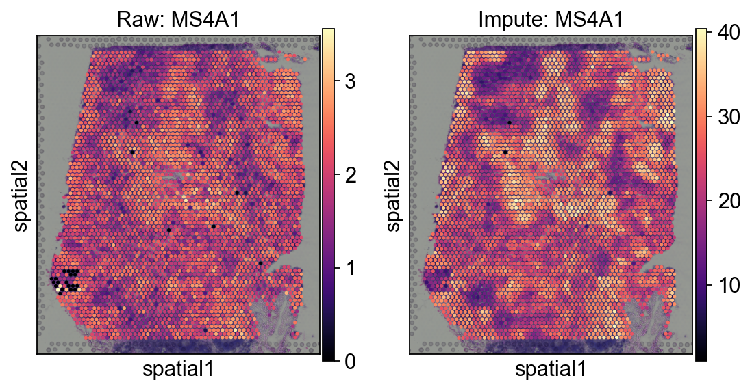
# fig = ov.plt.图(figsize=(4, 4))fig, 轴 = ov.plt.subplots(1,2,figsize=(8, 4))单细胞.pl.spatial(    decov_obj.adata_sp,     cmap='magma',    颜色='MS4A1',    ncols=4, 大小=1.3,ax=轴[0],    img_key='hires',显示=False,)轴[0].set_title('Raw: MS4A1')单细胞.pl.spatial(    decov_obj.adata_impute,     cmap='magma',    颜色='ms4a1',    ncols=4, 大小=1.3,ax=轴[1],    img_key='hires',显示=False,)轴[1].set_title('Impute: MS4A1')

Text(0.5, 1.0, 'Impute: MS4A1')

步骤 4: Cell2location 解卷积 (30–120 min, GPU recommended)Cell2location is a Bayesian model 那 resolves fine-grained 细胞类型 在 space. It typically proceeds 在 two stages:1) learn 参考 signatures 从 scRNA-seq; 2) map 那些 signatures 到 该 spatial sample 到 估计 细胞类型 abundances.

adata_sc = ov.datasets.sc_ref_Lymph_Node()adata_sp = sc.datasets.visium_sge(sample_id="V1_Human_Lymph_Node")adata_sp.obs['sample'] = list(adata_sp.uns['spatial'].keys())[0]adata_sp.var_names_make_unique()

reading /scratch/users/steorra/analysis/omic_test/data/V1_Human_Lymph_Node/filtered_feature_bc_matrix.h5
 (0:00:00)

decov_obj=ov.space.Deconvolution(    adata_sc=adata_sc,    adata_sp=adata_sp)

步骤 4.1 Run Cell2location

decov_obj.deconvolution(    method='cell2location',celltype_key_sc='Subset',    batch_key_sc=None,batch_key_sp='sample',    cell2location_scrna_kwargs={'max_epochs':200,'batch_size':2500,'train_size':1,'lr':0.002},    cell2location_spatial_kwargs={'max_epochs':20000,'batch_size':None,'train_size':1},    sample_kwargs={"num_samples": 1000, "batch_size": 2500})

INFO:lightning.pytorch.utilities.rank_zero:GPU available: True (cuda), used: True
INFO:lightning.pytorch.utilities.rank_zero:TPU available: False, using: 0 TPU cores
INFO:lightning.pytorch.utilities.rank_zero:HPU available: False, using: 0 HPUs
INFO:lightning.pytorch.utilities.rank_zero:You are using a CUDA device ('NVIDIA H100 80GB HBM3') that has Tensor Cores. To properly utilize them, you should set `torch.set_float32_matmul_precision('medium' | 'high')` which will trade-off precision for performance. For more details, read https://pytorch.org/docs/stable/generated/torch.set_float32_matmul_precision.html#torch.set_float32_matmul_precision
INFO:lightning.pytorch.accelerators.cuda:LOCAL_RANK: 0 - CUDA_VISIBLE_DEVICES: [0]
INFO:lightning.pytorch.utilities.rank_zero:`Trainer.fit` stopped: `max_epochs=200` reached.
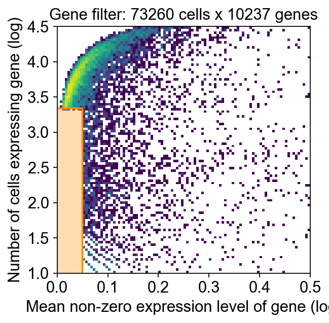
Total number of genes both in the scRNA-seq data and the spatial transcriptomics data: 10141
INFO:lightning.pytorch.utilities.rank_zero:GPU available: True (cuda), used: True
INFO:lightning.pytorch.utilities.rank_zero:TPU available: False, using: 0 TPU cores
INFO:lightning.pytorch.utilities.rank_zero:HPU available: False, using: 0 HPUs
INFO:lightning.pytorch.accelerators.cuda:LOCAL_RANK: 0 - CUDA_VISIBLE_DEVICES: [0]
INFO:lightning.pytorch.utilities.rank_zero:`Trainer.fit` stopped: `max_epochs=20000` reached.
✓ cell2location is done
The cell2location result is saved in self.adata_cell2location

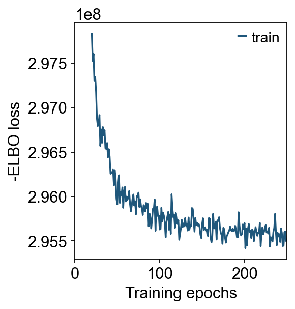
decov_obj.mod_sc.plot_history(20)ov.plt.show()decov_obj.mod_sp.plot_history(1000)

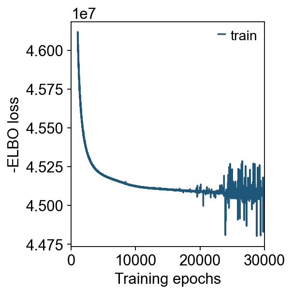
步骤 4.2 Spatial mapping 和 saving models (<1 min 到 保存)Recommended 到 保存 separately:- 参数/models 从 参考 learning- 参数/models 从 spatial mappingThis minimizes repeated training costs 在 future runs.

# 保存 model#ov.utils.保存(decov_obj.mod_sc,f"result/model/reference_signatures.pkl")# 保存 modelov.utils.保存(decov_obj.mod_sp,f"result/model/cell2location_map.pkl")

💾 Save Operation:
   Target path: result/model/reference_signatures.pkl
   Object type: RegressionModel
   Using: pickle
   Pickle failed, switching to: cloudpickle
   ✅ Successfully saved using cloudpickle!
────────────────────────────────────────────────────────────
💾 Save Operation:
   Target path: result/model/cell2location_map.pkl
   Object type: Cell2location
   Using: pickle
   Pickle failed, switching to: cloudpickle
   ✅ Successfully saved using cloudpickle!
────────────────────────────────────────────────────────────

decov_obj.adata_sc.write(f"result/model/cell2location_adata_sc.h5ad")decov_obj.adata_sp.write(f"result/model/cell2location_adata_sp.h5ad")

步骤 4.3 Result object: cell locations (Cell2location)

decov_obj.adata_cell2location

AnnData object with n_obs × n_vars = 4035 × 34
    obs: 'in_tissue', 'array_row', 'array_col', 'sample', '_indices', '_scvi_batch', '_scvi_labels'
    uns: 'spatial', '_scvi_uuid', '_scvi_manager_uuid', 'mod'
    obsm: 'spatial', 'means_cell_abundance_w_sf', 'stds_cell_abundance_w_sf', 'q05_cell_abundance_w_sf', 'q95_cell_abundance_w_sf', 'prop_celltypes'

步骤 4.4 Reuse: reload models 和 perform imputation

decov_obj=ov.space.Deconvolution(    adata_sc=ov.read(f"result/model/cell2location_adata_sc.h5ad"),    adata_sp=ov.read(f"result/model/cell2location_adata_sp.h5ad"),)decov_obj.load_cell2location_model(    mod_sp_path=f"result/model/cell2location_map.pkl")decov_obj.cell2location_inference()decov_obj.impute(method='cell2location')decov_obj.adata_sp

📂 Load Operation:
   Source path: result/model/cell2location_map.pkl
   Using: pickle
   ✅ Successfully loaded!
   Loaded object type: Cell2location
────────────────────────────────────────────────────────────
✓ cell2location model is loaded
The cell2location model is saved in self.mod_sc and self.mod_sp
INFO     AnnData object appears to be a copy. Attempting to transfer setup.
✓ cell2location is done
The cell2location result is saved in self.adata_cell2location
✓ cell2location impute is done
Compare with the tangram impute result, cell2location's impute stores in self.adata_sp.layers

AnnData object with n_obs × n_vars = 4035 × 10141
    obs: 'in_tissue', 'array_row', 'array_col', 'sample', '_indices', '_scvi_batch', '_scvi_labels'
    var: 'gene_ids', 'feature_types', 'genome'
    uns: '_scvi_manager_uuid', '_scvi_uuid', 'mod', 'spatial'
    obsm: 'means_cell_abundance_w_sf', 'prop_celltypes', 'q05_cell_abundance_w_sf', 'q95_cell_abundance_w_sf', 'spatial', 'stds_cell_abundance_w_sf'
    layers: 'B_Cycling', 'B_GC_DZ', 'B_GC_LZ', 'B_GC_prePB', 'B_IFN', 'B_activated', 'B_mem', 'B_naive', 'B_plasma', 'B_preGC', 'DC_CCR7+', 'DC_cDC1', 'DC_cDC2', 'DC_pDC', 'Endo', 'FDC', 'ILC', 'Macrophages_M1', 'Macrophages_M2', 'Mast', 'Monocytes', 'NK', 'NKT', 'T_CD4+', 'T_CD4+_TfH', 'T_CD4+_TfH_GC', 'T_CD4+_naive', 'T_CD8+_CD161+', 'T_CD8+_cytotoxic', 'T_CD8+_naive', 'T_TIM3+', 'T_TfR', 'T_Treg', 'VSMC'

# fig = ov.plt.图(figsize=(4, 4))fig, 轴 = ov.plt.subplots(1,2,figsize=(8, 4))单细胞.pl.spatial(    decov_obj.adata_sp,     cmap='magma',    颜色='MS4A1',    ncols=4, 大小=1.3,ax=轴[0],    img_key='hires',显示=False,)轴[0].set_title('Raw: MS4A1')单细胞.pl.spatial(    decov_obj.adata_sp,     layer='B_naive',    cmap='magma',    颜色='MS4A1',    ncols=4, 大小=1.3,ax=轴[1],    img_key='hires',显示=False,)轴[1].set_title('B_naive Impute: MS4A1')

Text(0.5, 1.0, 'B_naive Impute: MS4A1')

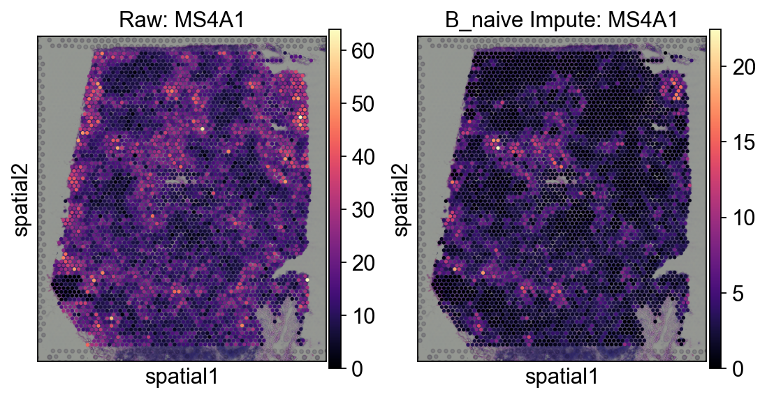
步骤 5: 可视化 (5–15 min)We provide multiple views: single-target spatial heatmaps, multi-target overlays, 和 local pie charts. Start 使用 global inspection, then zoom into biologically relevant regions 对于 higher-resolution assessment.### 5.1 Spatial value dotplot #### 5.1.1 Tangram

annotation_list=['B_Cycling', 'B_GC_LZ', 'T_CD4+_TfH_GC', 'FDC',                'B_naive', 'T_CD4+_naive', 'B_plasma', 'Endo']sc.pl.spatial(    decov_obj.adata_cell2location,     cmap='magma',    # 显示 first 8 细胞类型    颜色=annotation_list,    ncols=4, 大小=1.3,    img_key='hires',    # limit 颜色 缩放 在 99.2% quantile 的 cell abundance    #vmin=0, vmax='p99.2')

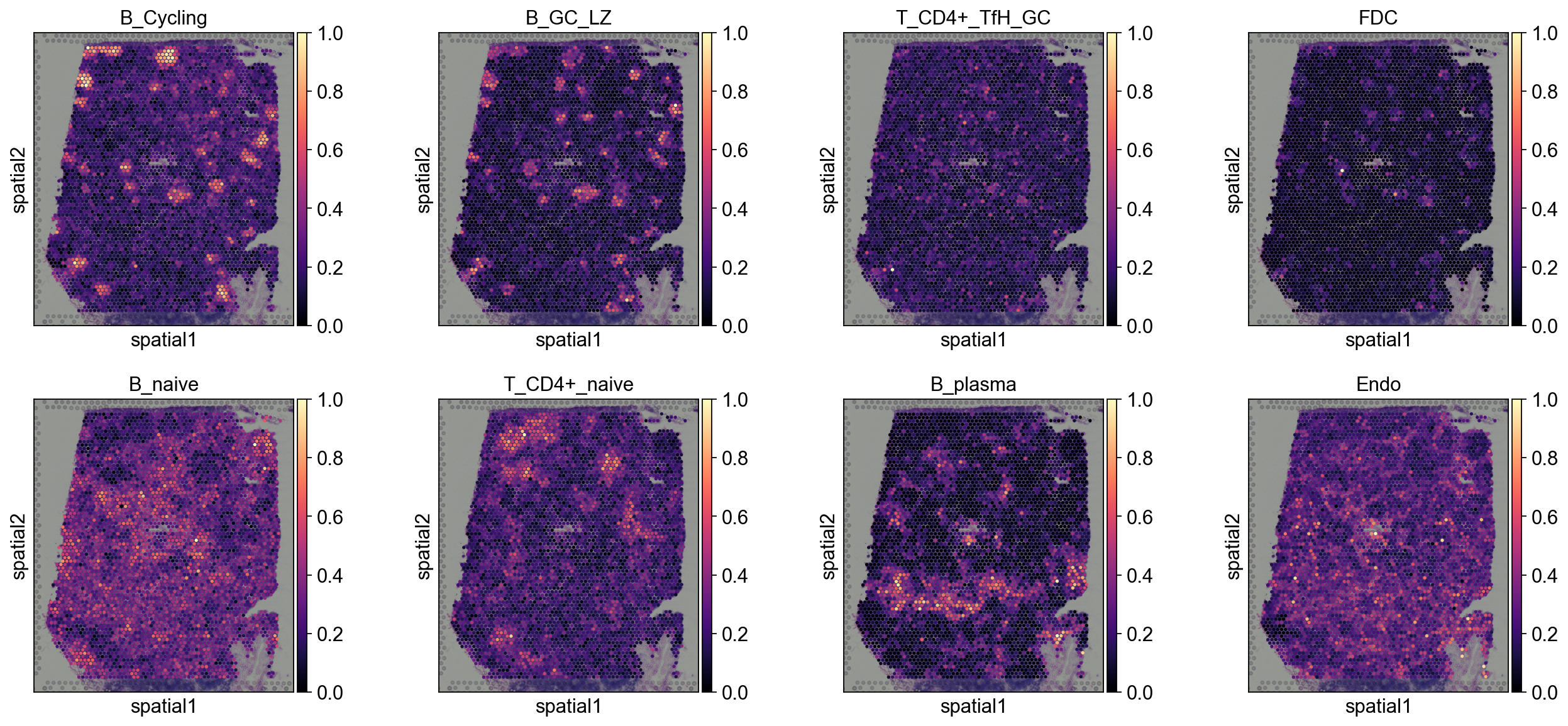
5.1.2 Cell2location

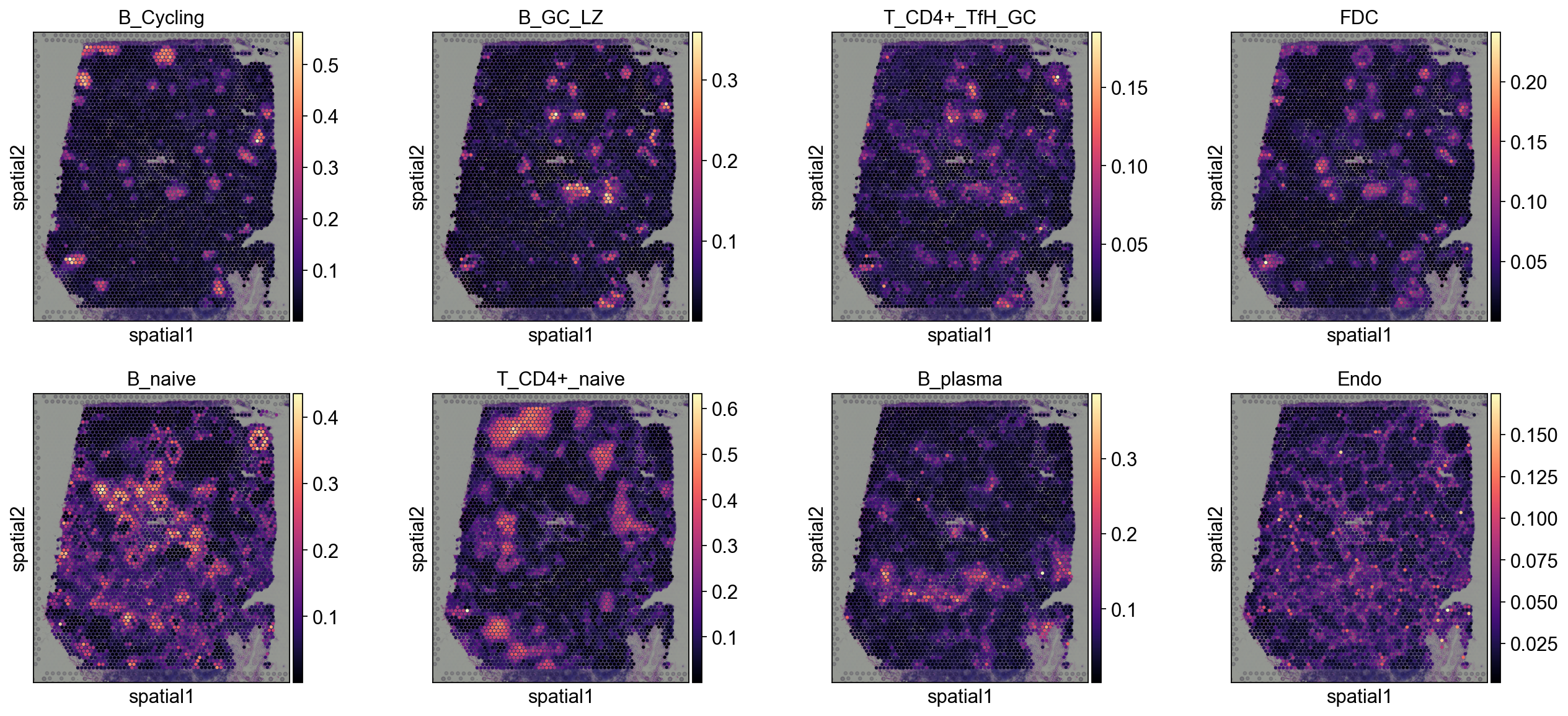
annotation_list=['B_Cycling', 'B_GC_LZ', 'T_CD4+_TfH_GC', 'FDC',                'B_naive', 'T_CD4+_naive', 'B_plasma', 'Endo']sc.pl.spatial(    decov_obj.adata_cell2location,     cmap='magma',    # 显示 first 8 细胞类型    颜色=annotation_list,    ncols=4, 大小=1.3,    img_key='hires',    # limit 颜色 缩放 在 99.2% quantile 的 cell abundance    #vmin=0, vmax='p99.2')

5.2 Multi-target overlay

color_dict=dict(zip(adata_sc.obs['Subset'].cat.categories,                   adata_sc.uns['Subset_colors']))

5.2.1 Tangram

import matplotlib as mplclust_labels = annotation_list[:5]clust_col = ['' + str(i) for i in clust_labels] # 在 case column names differ 从 labelswith mpl.rc_context({'图.figsize': (6, 6),'轴.grid': False}):    fig = ov.pl.plot_spatial(        adata=decov_obj.adata_cell2location,        # 标签 到 显示 在 a 绘制        颜色=clust_col, 标签=clust_labels,        show_img=True,        # 'fast' (white background) 或 'dark_background'        style='fast',        # limit 颜色 缩放 在 99.2% quantile 的 cell abundance        max_color_quantile=0.992,        # 大小 的 locations (adjust depending 在 图 大小)        circle_diameter=4,        reorder_cmap = [#0,            1,2,3,4,6], #['yellow', 'orange', 'blue', 'green', 'purple', 'grey', 'white'],        colorbar_position='right',        palette=color_dict    )

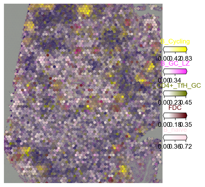
5.2.2 Cell2location

import matplotlib as mplclust_labels = annotation_list[:5]clust_col = ['' + str(i) for i in clust_labels] # 在 case column names differ 从 labelswith mpl.rc_context({'图.figsize': (6, 6),'轴.grid': False}):    fig = ov.pl.plot_spatial(        adata=decov_obj.adata_cell2location,        # 标签 到 显示 在 a 绘制        颜色=clust_col, 标签=clust_labels,        show_img=True,        # 'fast' (white background) 或 'dark_background'        style='fast',        # limit 颜色 缩放 在 99.2% quantile 的 cell abundance        max_color_quantile=0.992,        # 大小 的 locations (adjust depending 在 图 大小)        circle_diameter=4,        reorder_cmap = [#0,            1,2,3,4,6], #['yellow', 'orange', 'blue', 'green', 'purple', 'grey', 'white'],        colorbar_position='right',        palette=color_dict    )

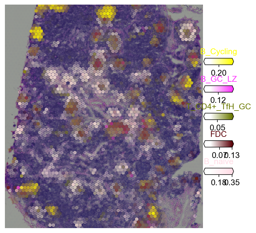
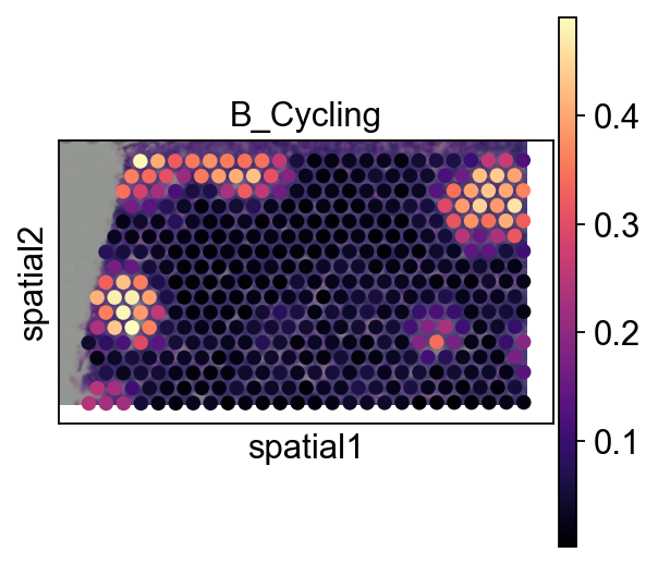
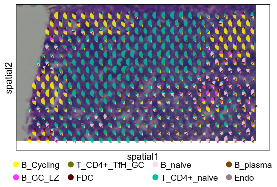
5.3 Pie plotWe recommend cropping a region 的 interest before plotting 到 avoid overly 密集 pie charts 在 whole slides.

adata_s = ov.space.crop_space_visium(    decov_obj.adata_cell2location,     crop_loc=(0, 0),          crop_area=(500, 1000),     library_id=list(decov_obj.adata_cell2location.uns['spatial'].keys())[0] ,     scale=1)

Adding image layer `image`

sc.pl.spatial(adata_s, cmap='magma',                  # 显示 first 8 细胞类型                  颜色=annotation_list[0],                  ncols=4, 大小=1.3,                  img_key='hires',                  # limit 颜色 缩放 在 99.2% quantile 的 cell abundance                  #vmin=0, vmax='p99.2'                 )

color_dict=dict(zip(adata_sc.obs['Subset'].cat.categories,                   adata_sc.uns['Subset_colors']))

5.3.1 Tangram

fig, ax = plt.subplots(figsize=(8, 4))sc.pl.spatial(    adata_s,     basis='spatial',    color=None,      size=1.3,    img_key='hires',    ax=ax,          show=False)ov.pl.add_pie2spatial(    adata_s,    img_key='hires',    cell_type_columns=annotation_list[:],    ax=ax,    colors=color_dict,    pie_radius=10,    remainder='gap',    legend_loc=(0.5, -0.25),    ncols=4,    alpha=0.8)plt.show()

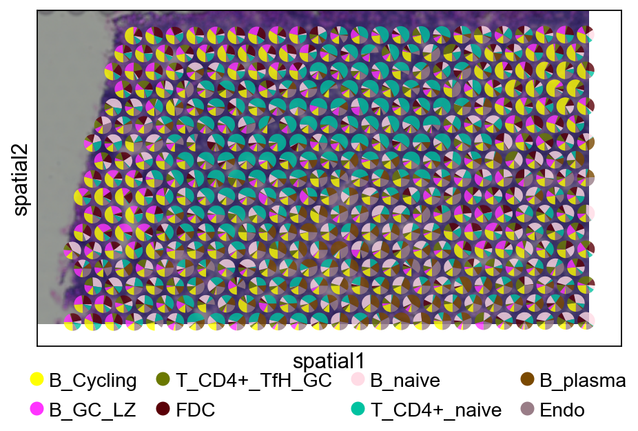
5.3.2 Cell2location

fig, ax = plt.subplots(figsize=(8, 4))sc.pl.spatial(    adata_s,     basis='spatial',    color=None,      size=1.3,    img_key='hires',    ax=ax,          show=False)ov.pl.add_pie2spatial(    adata_s,    img_key='hires',    cell_type_columns=annotation_list[:],    ax=ax,    colors=color_dict,    pie_radius=10,    remainder='gap',    legend_loc=(0.5, -0.25),    ncols=4,    alpha=0.8)plt.show()

Extensions 和 Further Reading- Cell2location official tutorials 和 docs: https://cell2location.readthedocs.io/en/latest/notebooks/cell2location_tutorial.html- Tangram paper 和 文档: consult official resources 对于 advanced 参数 和 updates.- Reproducibility tip: record omicverse 和 dependency versions 在 your project 对于 consistent results across 该 team.

from omicverse.external.space.cell2location.models import Cell2location, RegressionModelfrom omicverse.external.space.cell2location.plt import plot_spatialfrom omicverse.external.space.cell2location.utils import select_slidefrom omicverse.external.space.cell2location.utils.filtering import filter_genes

Citations 和 AcknowledgementsPlease cite:- OmicVerse toolkit (此 notebook’s implementation)- Tangram: original publication 和 software- Cell2location: original publication 和 software- 该 数据集 used (scRNA-seq 参考 和 空间转录组学)We thank 该 original tool authors 和 数据集 providers 对于 making their resources available 到 该 community.

import tangram as tg

Troubleshooting- 基因 ID mismatch: - Symptom: many NaNs 或 empty outputs; very few overlapping 基因. - Fix: harmonize 基因 IDs between scRNA-seq 和 spatial 数据 (ENSEMBL/symbols), drop non-overlapping 基因 和 log 计数.- 参考 coverage insufficient: - Symptom: expected 细胞类型 missing 在 known tissue regions. - Fix: augment 该 scRNA-seq 参考 使用 tissue/age/pathology-matched 数据; integrate multiple sources 和 correct batch effects.- Hyperparameters: - Tangram: pay attention 到 regularization 和 基因 selection; small grid search can help. - Cell2location: prefer GPU; adjust training epochs/priors 到 数据集 大小; monitor convergence diagnostics.- Reproducibility: - Fix random seeds 和 package versions; 保存 models 和 key intermediate artifacts; record environment details 在 该 top 的 该 notebook.