批量 RNA-seq 到单细胞 RNA-seqBulk2Single 用于批量 RNA-seq 反卷积。我们从 Bulk2Space 算法中提取了 beta-VAE 部分，并构建了一种可以从批量 RNA-seq 反卷积到单细胞 RNA-seq 的算法。此外，我们重新设计了数据的输入和输出，使其更兼容 Python 环境中的分析约定。Paper: De novo analysis of bulk RNA-seq data at spatially resolved single-cell resolutionCode: https://github.com/ZJUFanLab/bulk2spaceColab_Reproducibility：https://colab.research.google.com/drive/1He71hAyeAv1DHQyXUlxtoJ4QvwZwW7I0?usp=sharing本教程介绍了如何从批量 RNA-seq 和参考 scRNA-seq 数据中读取、设置和训练模型。我们使用 pdac 数据集作为示例

import scanpy as scimport omicverse as ovimport matplotlib.pyplot as pltov.plot_set()

____            _     _    __                  
  / __ \____ ___  (_)___| |  / /__  _____________ 
 / / / / __ `__ \/ / ___/ | / / _ \/ ___/ ___/ _ \ 
/ /_/ / / / / / / / /__ | |/ /  __/ /  (__  )  __/ 
\____/_/ /_/ /_/_/\___/ |___/\___/_/  /____/\___/                                              

Version: 1.6.3, Tutorials: https://omicverse.readthedocs.io/

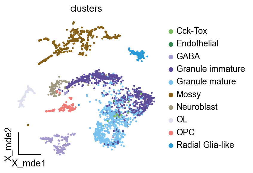
加载数据为了说明，我们对牙状回神经发生进行差异动力学分析，其包含多个异质亚群。我们利用从大鼠海马牙状回获得的单细胞 RNA-seq 数据 (GEO 编号: GSE95753) 以及批量 RNA-seq 数据 (GEO 编号: GSE74985)。

bulk_data=ov.read('data/GSE74985_mergedCount.txt.gz',index_col=0)bulk_data=ov.bulk.Matrix_ID_mapping(bulk_data,'genesets/pair_GRCm39.tsv')bulk_data.head()

	dg_d_1	dg_d_2	dg_d_3	dg_v_1	dg_v_2	dg_v_3	ca4_1	ca4_2	ca4_3	ca3_d_1	...	ca3_v_3	ca2_1	ca2_2	ca2_3	ca1_d_1	ca1_d_2	ca1_d_3	ca1_v_1	ca1_v_2	ca1_v_3
Gm12150	0	2	0	11	0	9	72	0	0	0	...	0	0	0	0	0	0	0	0	0	0
Mir219a-2	0	0	0	0	0	0	0	0	0	0	...	0	1	0	0	0	0	0	0	0	0
Hspd1	1418	685	1404	3073	2316	1945	7724	8255	6802	4956	...	8154	7104	5854	7508	5322	6172	5199	1865	1253	2298
Crhbp	0	0	0	31	17	32	0	0	0	29	...	0	0	1	0	0	0	0	0	0	0
Gm11735	0	0	0	0	0	0	0	0	0	0	...	0	0	0	0	0	0	0	0	0	0

5 rows × 24 columns

import anndataimport scvelo as scvsingle_data=scv.datasets.dentategyrus()single_data

AnnData object with n_obs × n_vars = 2930 × 13913
    obs: 'clusters', 'age(days)', 'clusters_enlarged'
    uns: 'clusters_colors'
    obsm: 'X_umap'
    layers: 'ambiguous', 'spliced', 'unspliced'

细胞比例计算我们现在可以设置 Bulk2Single 对象，这将确保模型所需的一切都准备好进行训练。我们需要指定 scRNA-seq 的细胞类型以反卷积批量 RNA-seq。并为每个细胞类型指定用于训练的标记基因数量。如果设置 gpu=-1，它将使用 CPU 配置 VAE 模型。

model=ov.bulk2single.Bulk2Single(bulk_data=bulk_data,single_data=single_data,                celltype_key='clusters',bulk_group=['dg_d_1','dg_d_2','dg_d_3'],                 top_marker_num=200,ratio_num=1,gpu=0)

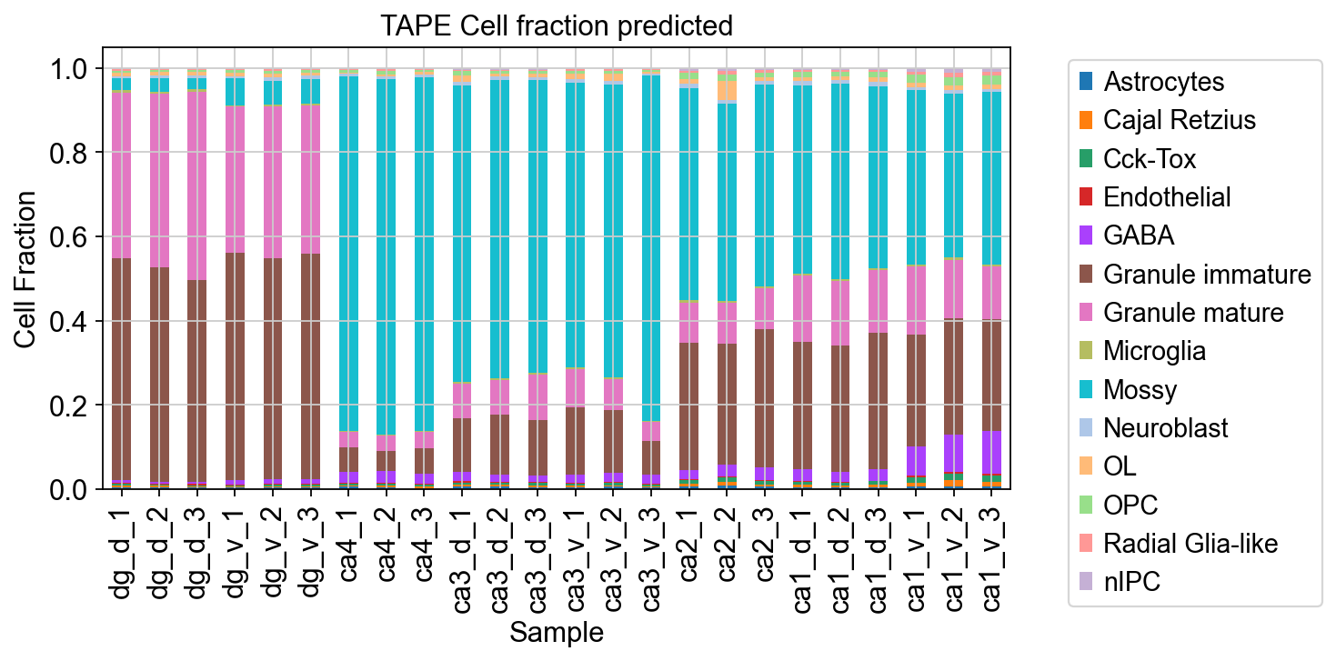
在这里，我们改进了 Bulk2space 中细胞比例的估计，并消除了原始作者使用的回归估计，这通常会导致比例出现较大偏差，正如我们的分析所证实的。我们引入了 TAPE，该模型能够准确地将批量 RNA-seq 数据反卷积为细胞分数，并基于 scRNA-seq 数据在细胞类型水平预测细胞类型特异性基因表达。Paper: Deep autoencoder for interpretable tissue-adaptive deconvolution and cell-type-specific gene analysisCode: poseidonchan/TAPE

CellFractionPrediction=model.predicted_fraction()

Reading single-cell dataset, this may take 1 min
Reading dataset is done
Normalizing raw single cell data with scanpy.pp.normalize_total
Generating cell fractions using Dirichlet distribution without prior info (actually random)
RANDOM cell fractions is generated
You set sparse as True, some cell's fraction will be zero, the probability is 0.5
Sampling cells to compose pseudo-bulk data
Sampling is done
Reading training data
Reading is done
Reading test data
Reading test data is done
Using counts data to train model
Cutting variance...
Finding intersected genes...
Intersected gene number is  12227
Scaling...
Using minmax scaler...
training data shape is  (5000, 12227) 
test data shape is  (24, 12227)
train model256 now
train model512 now
train model1024 now
Training of Scaden is done
Predicted Total Cell Num: 2457.268449380651

CellFractionPrediction.head()

	Astrocytes	Cajal Retzius	Cck-Tox	Endothelial	GABA	Granule immature	Granule mature	Microglia	Mossy	Neuroblast	OL	OPC	Radial Glia-like	nIPC
dg_d_1	0.004780	0.003839	0.004187	0.002460	0.005536	0.527208	0.393742	0.005203	0.028935	0.004639	0.007397	0.005216	0.002961	0.003898
dg_d_2	0.005013	0.002877	0.003001	0.002407	0.004481	0.508747	0.413222	0.004478	0.032327	0.006355	0.007488	0.004283	0.002102	0.003218
dg_d_3	0.003915	0.002676	0.002945	0.002558	0.005772	0.479360	0.446842	0.004949	0.026702	0.006624	0.008542	0.004052	0.002157	0.002908
dg_v_1	0.003247	0.002842	0.003309	0.001613	0.010134	0.539566	0.347792	0.002481	0.063813	0.006122	0.008335	0.005785	0.002116	0.002846
dg_v_2	0.004015	0.003188	0.003747	0.002137	0.010382	0.523644	0.362331	0.002693	0.056484	0.009367	0.008487	0.007403	0.002478	0.003644

我们使用堆积直方图来可视化每个样品的细胞比例

ax = CellFractionPrediction.plot(kind='bar', stacked=True, figsize=(8, 4))ax.set_xlabel('Sample')ax.set_ylabel('Cell Fraction')ax.set_title('TAPE Cell fraction predicted')plt.legend(bbox_to_anchor=(1.05, 1),ncol=1,)plt.show()

Bulk2single 训练### 预处理单细胞 RNA-seq 和批量 RNA-seq获得每个样品的细胞比例后，我们还想获得样品的单细胞数据，其中我们使用 beta-VAE 来预测批量数据中的细胞，我们首先对数据进行了预处理。这些组是 [‘dg_d_1’, ‘dg_d_2’, ‘dg_d_3’]，代表样品 DG 颗粒细胞

model.bulk_preprocess_lazy()model.single_preprocess_lazy()model.prepare_input()

......drop duplicates index in bulk data
......deseq2 normalize the bulk data
......log10 the bulk data
......calculate the mean of each group
......normalize the single data
normalizing counts per cell
    finished (0:00:00)
......log1p the single data
......prepare the input of bulk2single
...loading data

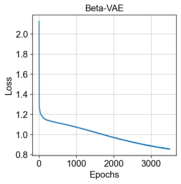
训练 VAE 模型我们开始训练 VAE 模型以生成单细胞数据，该过程在 CPU 上花费约 3 小时，在 GPU 上仅需 10 分钟。

Note

默认最大周期设置为 3500，但实际上 Bulk2Single 一旦模型收敛就会提前停止，这很少需要那么多，特别是对于大型数据集。(我们可以设置 patience 来控制停止步骤)

vae_net=model.train(    batch_size=512,    learning_rate=1e-4,    hidden_size=256,    epoch_num=3500,    vae_save_dir='data/bulk2single/save_model',    vae_save_name='dg_vae',    generate_save_dir='data/bulk2single/output',    generate_save_name='dg')

...begin vae training
min loss = 0.8544222712516785
...vae training done!
...save trained vae in data/bulk2single/save_model/dg_vae.pth.

我们可以使用名为 plot_loss 的简单方法绘制 vae 损失

model.plot_loss()

(<Figure size 320x320 with 1 Axes>,
 <AxesSubplot: title={'center': 'Beta-VAE'}, xlabel='Epochs', ylabel='Loss'>)

我们也可以直接加载我们之前训练的模型

# model.load_fraction('dg_vae_cell_target_num.pkl')#model.bulk_preprocess_lazy()#model.single_preprocess_lazy()#model.prepare_input()vae_net=model.load('data/bulk2single/save_model/dg_vae.pth')

......drop duplicates index in bulk data
......deseq2 normalize the bulk data
......log10 the bulk data
......calculate the mean of each group
......normalize the single data
normalizing counts per cell
    finished (0:00:00)
......log1p the single data
......prepare the input of bulk2single
...loading data
loading model from data/bulk2single/save_model/dg_vae.pth

现在，我们可以从我们的模型生成一个 Bulk2Single 反卷积的 scRNA-seq 矩阵。

generate_adata=model.generate()generate_adata

...generating
generated done!

AnnData object with n_obs × n_vars = 4907 × 12953
    obs: 'clusters'

我们直接生成的单细胞数据中存在大量噪声，我们需要过滤嘈杂的细胞。

generate_adata=model.filtered(generate_adata,leiden_size=25)generate_adata

extracting highly variable genes
    finished (0:00:00)
--> added
    'highly_variable', boolean vector (adata.var)
    'means', float vector (adata.var)
    'dispersions', float vector (adata.var)
    'dispersions_norm', float vector (adata.var)
computing PCA
Note that scikit-learn's randomized PCA might not be exactly reproducible across different computational platforms. For exact reproducibility, choose `svd_solver='arpack'.`
    on highly variable genes
    with n_comps=100
    finished (0:00:02)
computing neighbors
    finished: added to `.uns['neighbors']`
    `.obsp['distances']`, distances for each pair of neighbors
    `.obsp['connectivities']`, weighted adjacency matrix (0:00:02)
running Leiden clustering
    finished: found 129 clusters and added
    'leiden', the cluster labels (adata.obs, categorical) (0:00:00)
The filter leiden is  ['22', '43', '38', '39', '40', '41', '42', '45', '44', '46', '47', '48', '36', '37', '30', '35', '28', '23', '34', '25', '26', '27', '24', '29', '31', '32', '33', '49', '50', '51', '52', '53', '54', '61', '66', '65', '63', '62', '64', '60', '58', '57', '56', '55', '59', '87', '83', '84', '85', '86', '90', '88', '89', '81', '91', '92', '93', '82', '78', '80', '79', '77', '76', '75', '74', '73', '72', '71', '70', '69', '68', '67', '94', '95', '96', '108', '118', '117', '116', '115', '114', '113', '97', '111', '110', '109', '112', '107', '105', '104', '103', '102', '101', '100', '99', '98', '106', '122', '124', '123', '119', '121', '120', '125', '126', '127', '128']

View of AnnData object with n_obs × n_vars = 3591 × 1529
    obs: 'clusters', 'leiden'
    var: 'highly_variable', 'means', 'dispersions', 'dispersions_norm', 'mean', 'std'
    uns: 'hvg', 'pca', 'neighbors', 'leiden'
    obsm: 'X_pca'
    varm: 'PCs'
    obsp: 'distances', 'connectivities'

可视化和分析相关性我们需要测试生成的单细胞 RNA-seq 的特性及其与参考 scRNA-seq 的相关性。在这里，我们使用参考 scRNA-seq 的细胞类型特异性标记作为锚点，使用皮尔逊系数计算了参考 scRNA-seq 的细胞类型与生成的 scRNA-seq 的细胞类型之间的相关性。

ov.bulk2single.bulk2single_plot_cellprop(generate_adata,celltype_key='clusters')plt.grid(False)

我们很容易比较参考 scRNA-seq 和生成的 scRNA-seq 之间的细胞比例

ov.bulk2single.bulk2single_plot_cellprop(single_data,celltype_key='clusters')plt.grid(False)

ov.bulk2single.bulk2single_plot_correlation(single_data,generate_adata,celltype_key='clusters')plt.grid(False)

ranking genes
    finished: added to `.uns['rank_genes_groups']`
    'names', sorted np.recarray to be indexed by group ids
    'scores', sorted np.recarray to be indexed by group ids
    'logfoldchanges', sorted np.recarray to be indexed by group ids
    'pvals', sorted np.recarray to be indexed by group ids
    'pvals_adj', sorted np.recarray to be indexed by group ids (0:00:01)

import scanpy as scgenerate_adata.obsm["X_mde"] = ov.utils.mde(generate_adata.obsm["X_pca"])ov.pl.embedding(generate_adata,basis='X_mde',color=['clusters'],wspace=0.4,          palette=ov.utils.pyomic_palette(),frameon='small')