使用 LIANA+ 进行细胞通讯分析

概览

本教程围绕 LIANA+ 的 rank_aggregate 工作流展开，并把结果统一接到 OmicVerse 的 ccc_* 可视化体系。

1. ov.pl.ccc_heatmap

2. ov.pl.ccc_network_plot

3. ov.pl.ccc_stat_plot

这样做的目的，是先建立“同一份通讯结果可以从哪些角度解释”的整体框架，再进入具体图形。

同时本教程保留两条思路：

• 主流程：直接把原始 adata 传给 ccc_*

• 可选流程：显式提取 comm_adata，便于结果检查和构造比较示例

方法背景

参考 LIANA 官方文档 和 LIANA+ 论文，LIANA+ 是一个统一不同配体-受体资源与多种打分策略的细胞通讯分析框架。

本教程重点展示 rank_aggregate，因为它很适合作为默认入口：

• 根据细胞标签定义 sender 和 receiver 群体

• 基于标准化表达模式为配体-受体相互作用打分

• 对多种方法的结果进行综合，得到共识排序

• 返回标准化结果表，方便接入 OmicVerse 的 ccc_* 可视化函数

这种“先做共识排序，再做下游解释”的思路，适合需要先筛选候选通讯轴、再进入 pathway 或 network 解释的场景。

为什么这里使用 pbmc68k_reduced？

pbmc68k_reduced 数据量轻、已经带有 UMAP 坐标，并且包含数量适中的免疫细胞群，因此既能完整演示 LIANA+ 推断流程，也能让后续通讯图保持可读性。

import numpy as np
import pandas as pd
import scanpy as sc
import warnings
warnings.filterwarnings("ignore", category=FutureWarning)

import omicverse as ov

ov.plot_set(font_path='Arial')

%reload_ext autoreload
%autoreload 2

🔬 Starting plot initialization...
Using already downloaded Arial font from: /var/folders/rv/3jnfbs0d6r7d0c5bfj7ft5k00000gn/T/omicverse_arial.ttf
Registered as: Arial
🧬 Detecting GPU devices…
✅ Apple Silicon MPS detected
    • [MPS] Apple Silicon GPU - Metal Performance Shaders available

   ____            _     _    __                  
  / __ \____ ___  (_)___| |  / /__  _____________ 
 / / / / __ `__ \/ / ___/ | / / _ \/ ___/ ___/ _ \ 
/ /_/ / / / / / / / /__ | |/ /  __/ /  (__  )  __/ 
\____/_/ /_/ /_/_/\___/ |___/\___/_/  /____/\___/                                              

🔖 Version: 2.1.3rc1   📚 Tutorials: https://omicverse.readthedocs.io/
✅ plot_set complete.

1. 载入示例数据

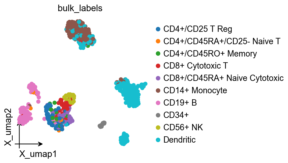
LIANA 官方教程同样基于 AnnData 工作流。这里使用 pbmc68k_reduced，并把 adata.obs['bulk_labels'] 作为通讯分组。

选择这个数据集的原因是：

• 足够轻量，便于完整展示多个 ccc_* 视图

• 已有 UMAP，可直接用于网络布局和结果检查

• 细胞类型数量适中，既能看到分面结构，也不会让图完全失控

adata = sc.datasets.pbmc68k_reduced()
adata

AnnData object with n_obs × n_vars = 700 × 765
    obs: 'bulk_labels', 'n_genes', 'percent_mito', 'n_counts', 'S_score', 'G2M_score', 'phase', 'louvain'
    var: 'n_counts', 'means', 'dispersions', 'dispersions_norm', 'highly_variable'
    uns: 'bulk_labels_colors', 'louvain', 'louvain_colors', 'neighbors', 'pca', 'rank_genes_groups'
    obsm: 'X_pca', 'X_umap'
    varm: 'PCs'
    obsp: 'distances', 'connectivities'

ov.pl.embedding(
    adata,
    basis='X_umap',
    color='bulk_labels',
    frameon='small'
)

2. 运行 LIANA+ rank aggregation

这里使用 ov.single.run_liana(...) 对 liana.mt.rank_aggregate 做封装，并把结果写到 adata.uns['liana_res']。

为什么这里默认选择 method='rank_aggregate'：

• aggregate 后的共识分数最适合接 OmicVerse 统一的 ccc_* 可视化

• 它能把多种 CCC 方法的证据折叠成一个排序结果，更适合作为教程的默认入口

• 后续无论是 interaction 级还是 pathway 级图，都可以围绕这张结果表继续组织

ov.single.run_liana(
    adata,
    groupby='bulk_labels',
    method='rank_aggregate',
    resource_name='consensus',
    key_added='liana_res',
    inplace=True,
)

adata.uns['liana_res'].head()

         source                      target ligand_complex receptor_complex  \
1209  Dendritic         CD4+/CD45RO+ Memory        HLA-DRA              CD4   
1188  Dendritic  CD4+/CD45RA+/CD25- Naive T        HLA-DRA              CD4   
1210  Dendritic         CD4+/CD45RO+ Memory       HLA-DRB1              CD4   
1205  Dendritic         CD4+/CD45RO+ Memory       HLA-DPB1              CD4   
1189  Dendritic  CD4+/CD45RA+/CD25- Naive T       HLA-DRB1              CD4   

      lr_means  cellphone_pvals  expr_prod  scaled_weight  lr_logfc  \
1209  2.575263              0.0   2.780884       0.723815  1.431303   
1188  2.566905              0.0   2.705027       0.709428  1.332656   
1210  2.415010              0.0   2.584465       0.712731  1.331341   
1205  2.367473              0.0   2.526199       0.731297  1.447014   
1189  2.406652              0.0   2.513965       0.698344  1.232695   

      spec_weight   lrscore  specificity_rank  magnitude_rank  
1209     0.065077  0.736772          0.001137        0.000653  
1188     0.063302  0.734081          0.001137        0.000911  
1210     0.060203  0.729607          0.001137        0.001211  
1205     0.068953  0.727352          0.001137        0.001377  
1189     0.058561  0.726870          0.001137        0.001741  

3. 可选：提取标准化后的通信 AnnData

现在大多数 ccc_* 调用已经不需要手动先构建 comm_adata，因为绘图函数会自动识别 adata.uns['liana_res']。

这里仍然显式提取一次，原因有三个：

1. 检查 LIANA 列如何被映射为标准通信 score / pvalue

2. 检查 pathway/classification 是否补齐

3. 后面构造 synthetic comparison、差异网络示例时，直接操作 comm_adata 更方便

comm_adata = ov.single.to_comm_adata(
    adata,
    result_uns_key='liana_res',
    score_key='specificity_rank',
    pvalue_key='specificity_rank',
    classification_reference='cellchat',
    classification_fallback='family',
)

comm_adata

AnnData object with n_obs × n_vars = 100 × 42
    obs: 'sender', 'receiver', 'cell_type_pair'
    var: 'interacting_pair', 'pair_lr', 'interaction_name', 'interaction_name_2', 'classification', 'pathway_name', 'signaling', 'gene_a', 'gene_b', 'ligand', 'receptor', 'annotation_strategy', 'classification_source'
    uns: 'liana_score_key', 'liana_pvalue_key', 'liana_uns_key', 'liana_sample_key', 'liana_classification_reference', 'liana_classification_fallback', 'liana_classification_source_counts'
    layers: 'means', 'pvalues', 'lr_means', 'cellphone_pvals', 'expr_prod', 'scaled_weight', 'lr_logfc', 'spec_weight', 'lrscore', 'specificity_rank', 'magnitude_rank'

comm_adata.var[['classification', 'classification_source']].value_counts().head()

classification  classification_source   
MHC-II          reference:cellchat_human    10
                family                       8
ECM/Adhesion    family                       6
Unclassified    unclassified                 5
TNF             family                       3
Name: count, dtype: int64

focus_pathways = [
    value
    for value in comm_adata.var['classification'].dropna().astype(str).unique().tolist()
    if value not in {'Unclassified', 'nan'}
]
focus_pathway = focus_pathways[0] if focus_pathways else 'Unclassified'
focus_pair_lr = comm_adata.var['interacting_pair'].astype(str).iloc[10]
ligand_series = comm_adata.var['ligand'].astype(str)
focus_ligand = ligand_series[ligand_series != ''].iloc[0]

color_dict = dict(
    zip(
        sorted(adata.obs['bulk_labels'].astype(str).unique()),
        ov.pl.sc_color[: adata.obs['bulk_labels'].nunique()],
    )
)

umap_df = pd.DataFrame(
    adata.obsm['X_umap'][:, :2],
    columns=['x', 'y'],
    index=adata.obs_names,
)
umap_df['cell_type'] = adata.obs['bulk_labels'].astype(str).values
node_positions = umap_df.groupby('cell_type', observed=True)[['x', 'y']].median()
embedding_points = umap_df.reset_index(drop=True)
comm_adata.uns['node_positions'] = node_positions
comm_adata.uns['embedding_points'] = embedding_points
comm_adata.uns['embedding_axes'] = ('UMAP_1', 'UMAP_2')

comparison_comm = comm_adata.copy()
comparison_comm.layers['means'] = np.asarray(comm_adata.layers['means']).copy() * 0.85
comparison_comm.layers['pvalues'] = np.clip(
    np.asarray(comm_adata.layers['pvalues']).copy() * 1.1,
    0.0,
    1.0,
)

focus_pathway, focus_pair_lr, focus_ligand

('ANNEXIN', 'HLA-DPA1_CD4', 'ANXA1')

一、ov.pl.ccc_heatmap

这一组图主要回答三个问题：

• 哪些 sender / receiver / interaction 组合最重要

• pathway 聚合后，哪些 signaling family 最活跃

• 在高密度矩阵里，哪些模式更适合做压缩展示

对 LIANA 而言，最值得优先掌握的是：

• plot_type='dot'：source-target-interaction 三层结构最清楚

• plot_type='tile'：左右拆开看 ligand / receptor 侧

• plot_type='sample_dot'：比较不同 context / sample 下的同一批 interaction

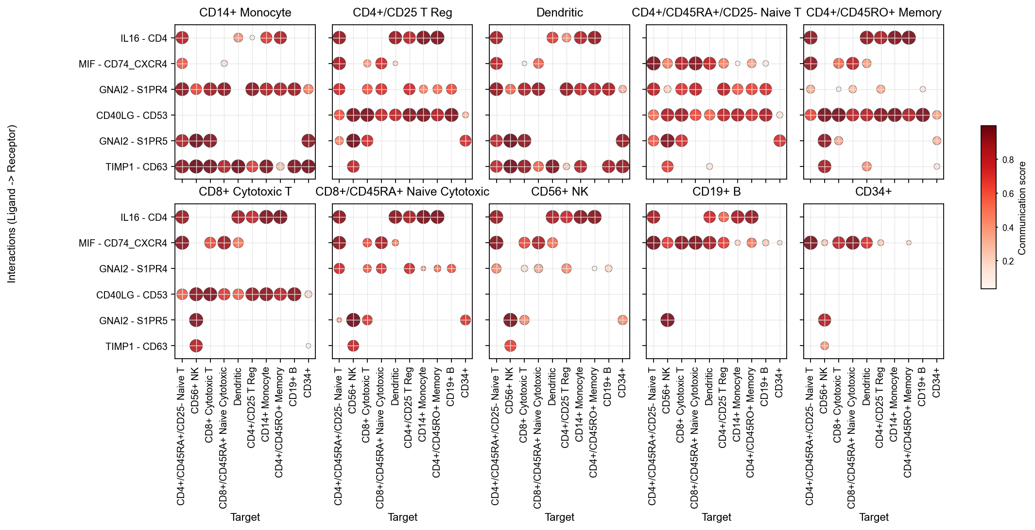
1.1 LIANA 主 dot 视图

这张图应该作为 interaction-level 的首选入口。

• 分面：source

• x 轴：target

• y 轴：interaction

• 颜色：communication score

可以清晰地查看 sender / target / interaction 三层信息。

fig, ax = ov.pl.ccc_heatmap(
    adata,
    plot_type='dot',
    display_by='interaction',
    score_key='specificity_rank',
    pvalue_key='specificity_rank',
    classification_reference='cellchat',
    classification_fallback='family',
    top_n=6,
    pvalue_threshold=0.05,
    color_by='score',
    ncols=5,
    figsize=(16, 5),
    show=False,
)

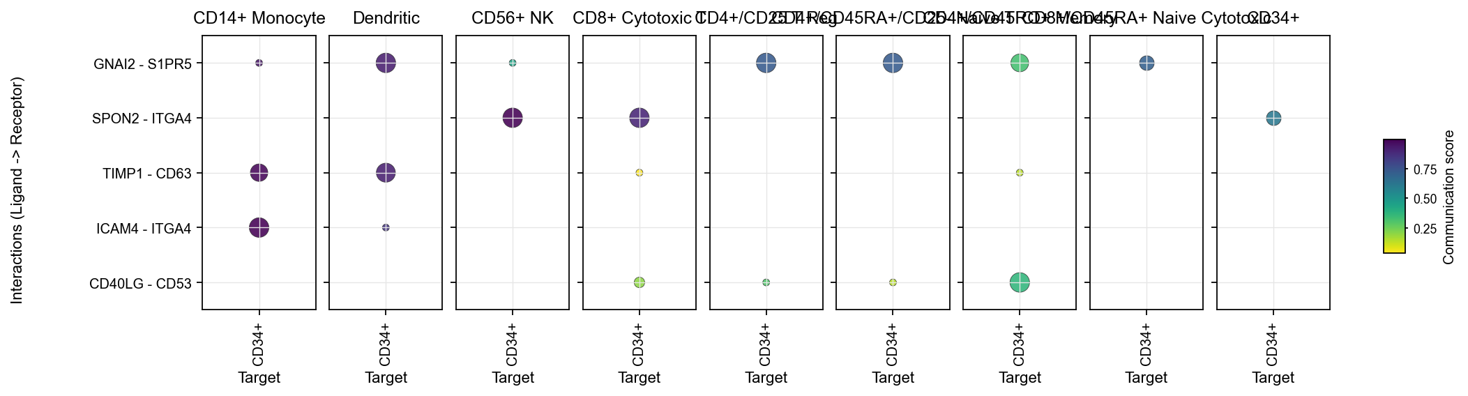
1.2 sender 聚焦 dot

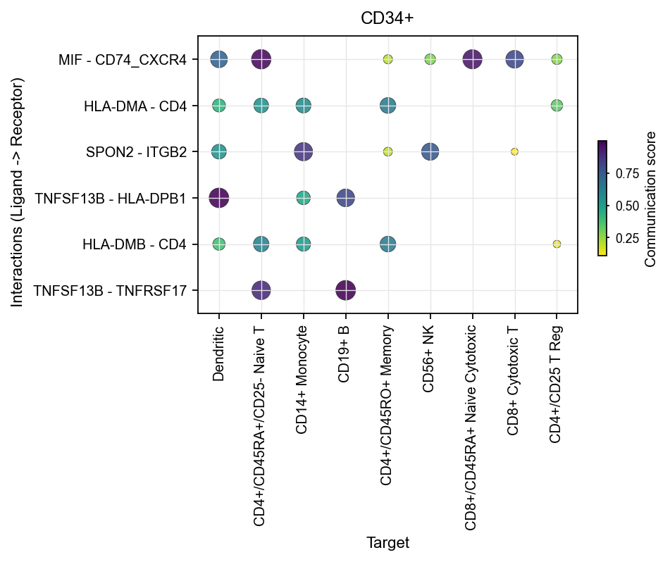
当你已经知道要看哪个 sender 时，可以直接用 sender_use 收窄范围。

这类图适合回答：

• 某个 sender 主要打向哪些 target

• 该 sender 的前几个 interaction 是什么

这里使用 ov.single.to_comm_adata 提取得到的 comm_adata 进行绘图，以 CD34+ 为例：

fig, ax = ov.pl.ccc_heatmap(
    comm_adata,
    plot_type='dot',
    display_by='interaction',
    score_key='specificity_rank',
    pvalue_key='specificity_rank',
    sender_use='CD34+',
    top_n=6,
    pvalue_threshold=0.05,
    color_by='score',
    cmap='viridis_r',
    figsize=(6, 3),
    show=False,
)

同样，也可以设置感兴趣的receiver_use

fig, ax = ov.pl.ccc_heatmap(
    adata,
    plot_type='dot',
    display_by='interaction',
    score_key='specificity_rank',
    pvalue_key='specificity_rank',
    receiver_use='CD34+',
    top_n=5,
    pvalue_threshold=0.05,
    color_by='score',
    cmap='viridis_r',
    figsize=(16, 3),
    show=False,
)

1.3 tile 图

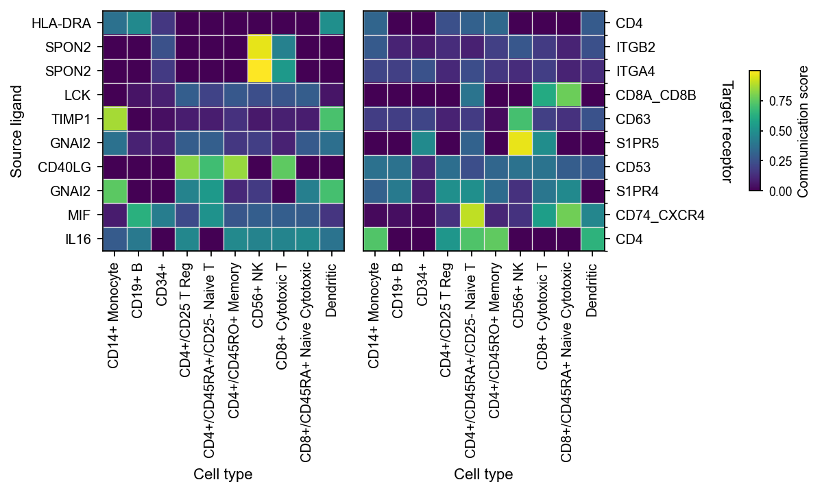
tile 适合在同一批 interaction 上，拆开看 ligand 侧和 receptor 侧分别落在哪些细胞群。

• 左热图：Source ligand

• 右热图：Target receptor

fig, ax = ov.pl.ccc_heatmap(
    adata,
    plot_type='tile',
    display_by='interaction',
    score_key='specificity_rank',
    pvalue_key='specificity_rank',
    top_n=10,
    pvalue_threshold=0.05,
    cmap='viridis',
    figsize=(8, 3),
    show=False,
)

1.4 pathway aggregation heatmap

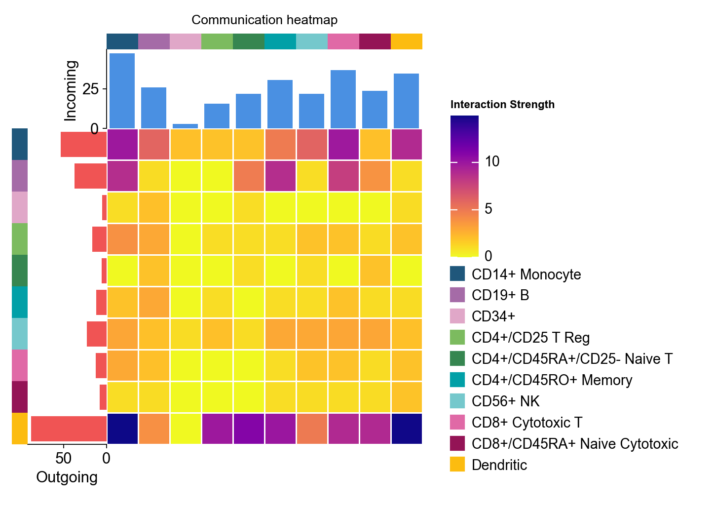
当问题从“哪个 interaction 最强”切换成“哪个 signaling family 最活跃”时，可以切换到 aggregation 级视图。

这里 classification_reference='cellchat' 和 classification_fallback='family' 才真正重要，因为它们决定了 pair 如何被归入 pathway/family。

fig, ax = ov.pl.ccc_heatmap(
    adata,
    plot_type='heatmap',
    display_by='aggregation',
    score_key='specificity_rank',
    pvalue_key='specificity_rank',
    classification_reference='cellchat',
    classification_fallback='family',
    top_n=12,
    cmap='plasma_r',
    show=False,
)

1.5 focused heatmap

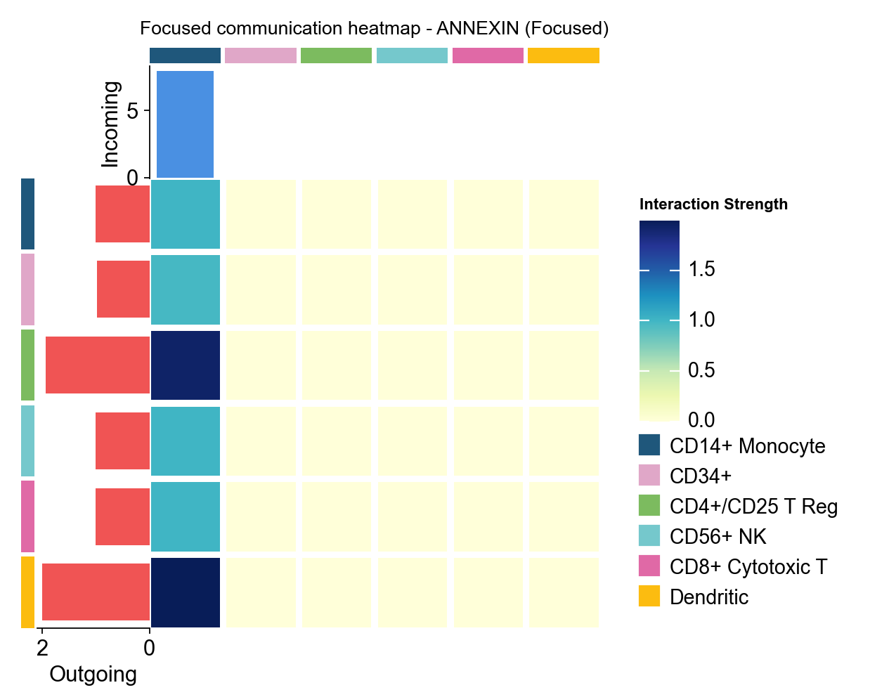
focused_heatmap 用于把某个 pathway 拉出来单独看 sender/receiver 的强弱格局。

fig, ax = ov.pl.ccc_heatmap(
    adata,
    plot_type='focused_heatmap',
    signaling=[focus_pathway],
    min_interaction_threshold=0.0,
    cmap='YlGnBu',
    figsize=(4, 3),
    show=False,
)

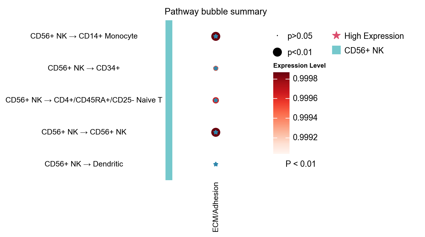
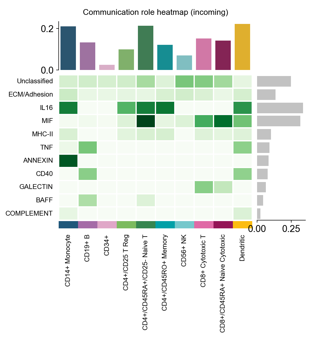
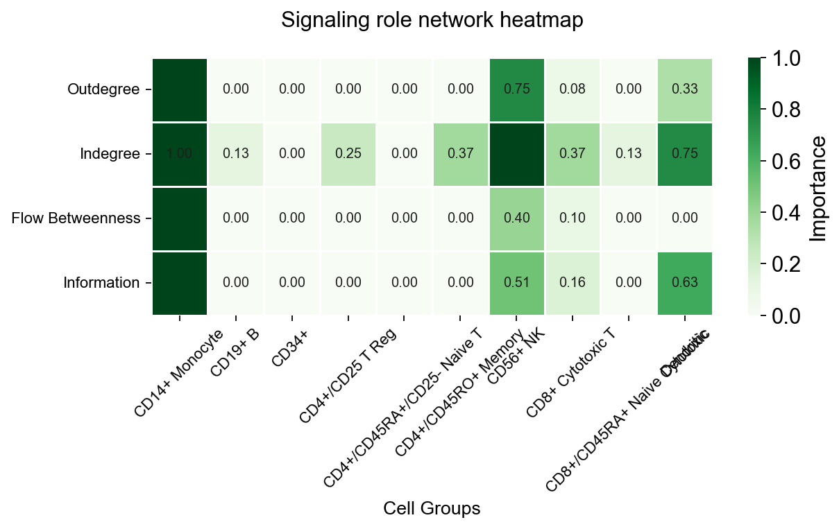
1.6 pathway bubble / role heatmap / role network

这三类图都偏 pathway-level summary：

• pathway_bubble：看 pathway 与 cell-pair 的紧凑矩阵

• role_heatmap：看 incoming / outgoing 模式

• role_network：把 pathway 角色关系再组织成网络

fig, ax = ov.pl.ccc_heatmap(
    comm_adata,
    plot_type='pathway_bubble',
    signaling=['ECM/Adhesion'],
    top_n=5,
    figsize=(3, 5),
    show=False,
)

📊 Visualization statistics:
   - Number of significant interactions: 5
   - Number of cell type pairs: 5
   - Signaling pathways: 1
   - Data scaling: None (raw expression values)
   - Color bars: sender

fig, ax = ov.pl.ccc_heatmap(
    adata,
    plot_type='role_heatmap',
    pattern='incoming',
    cmap='Greens',
    figsize=(4, 3),
    show=False,
)

🔬 Calculating cell communication strength for 11 pathways...
   - Aggregation method: mean
   - Minimum expression threshold: 0.1
✅ Completed pathway communication strength calculation for 11 pathways
📊 Pathway significance analysis results:
   - Total pathways: 11
   - Significant pathways: 11
   - Strength threshold: 0.5
   - p-value threshold: 0.05

🏆 Top 10 pathways by total strength:
----------------------------------------------------------------------------------------------------
Pathway                        Total    Max     Mean    L-R  Active Sig  Rate   Status
----------------------------------------------------------------------------------------------------
Unclassified                   58.62    0.99    0.72    5    81     33   0.41   ***
ECM/Adhesion                   35.78    1.00    0.76    6    47     25   0.53   ***
IL16                           33.61    0.98    0.86    1    39     10   0.26   ***
MIF                            31.59    0.98    0.64    1    49     5    0.10   ***
MHC-II                         22.20    1.00    0.69    18   32     16   0.50   ***
TNF                            20.53    1.00    0.89    3    23     14   0.61   ***
ANNEXIN                        8.82     1.00    0.88    2    10     6    0.60   ***
CD40                           7.79     1.00    0.97    1    8      7    0.88   ***
GALECTIN                       6.39     1.00    0.58    1    11     4    0.36   ***
BAFF                           5.83     1.00    0.97    2    6      5    0.83   ***
📊 Heatmap statistics:
   - Number of pathways: 11
   - Number of cell types: 10
   - Signal strength range: 0.000 - 0.900

fig, ax = ov.pl.ccc_heatmap(
    adata,
    plot_type='role_network',
    signaling=['ECM/Adhesion'],
    cmap='Greens',
    figsize=(8, 5),
    show=False,
)

✅ Network centrality calculation completed (CellChat-style Importance values)
   - Signaling pathways used: ['ECM/Adhesion']
   - Weight mode: Weighted
   - Calculated metrics: outdegree, indegree, flow_betweenness, information, overall
   - All centrality scores normalized to 0-1 range (Importance values)
📊 Signaling role analysis results (Importance values 0-1):
   - Dominant Sender: CD14+ Monocyte (Importance: 1.000)
   - Dominant Receiver: CD56+ NK (Importance: 1.000)
   - Mediator: CD14+ Monocyte (Importance: 1.000)
   - Influencer: CD14+ Monocyte (Importance: 1.000)

1.7 sample/context dot

sample_dot 需要 LIANA 结果表里有一个 context/sample 维度。

这里先用教程式的 synthetic condition 演示 API：复制同一份 liana_res 两份，并人为添加 baseline / stimulated。

这一步只是为了展示图形，不代表真实条件比较分析。

adata_by_context = adata.copy()
frames = []
for condition, delta in [('baseline', 0.0), ('stimulated', 0.03)]:
    frame = adata.uns['liana_res'].copy()
    frame['condition'] = condition
    frame['specificity_rank'] = np.clip(frame['specificity_rank'] + delta, 0.0, 1.0)
    frames.append(frame)
adata_by_context.uns['liana_res'] = pd.concat(frames, ignore_index=True)

fig, ax = ov.pl.ccc_heatmap(
    adata_by_context,
    plot_type='sample_dot',
    display_by='interaction',
    score_key='specificity_rank',
    pvalue_key='specificity_rank',
    sample_key='condition',
    top_n=3,
    top_n_pairs=6,
    pvalue_threshold=0.05,
    figsize=(9, 3),
    show=False,
)

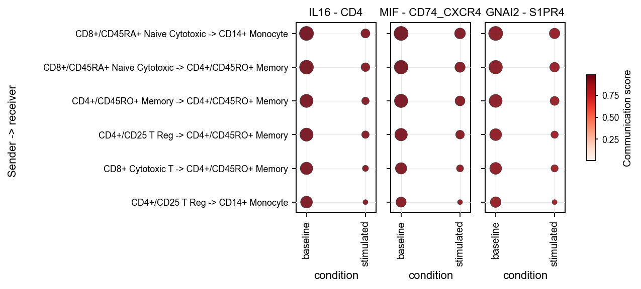
如果你有真实 condition 列，应该按条件分别运行 LIANA，再把不同条件的结果表合并后传给 sample_dot。下面给出一个最小 workflow 模板。

# condition_key = 'condition'
# result_frames = []
# for condition in sorted(adata.obs[condition_key].dropna().astype(str).unique()):
#     ad_sub = adata[adata.obs[condition_key].astype(str) == condition].copy()
#     ov.single.run_liana(
#         ad_sub,
#         groupby='bulk_labels',
#         method='rank_aggregate',
#         key_added='liana_res',
#         inplace=True,
#     )
#     frame = ad_sub.uns['liana_res'].copy()
#     frame[condition_key] = condition
#     result_frames.append(frame)
# adata_real_context = adata.copy()
# adata_real_context.uns['liana_res'] = pd.concat(result_frames, ignore_index=True)

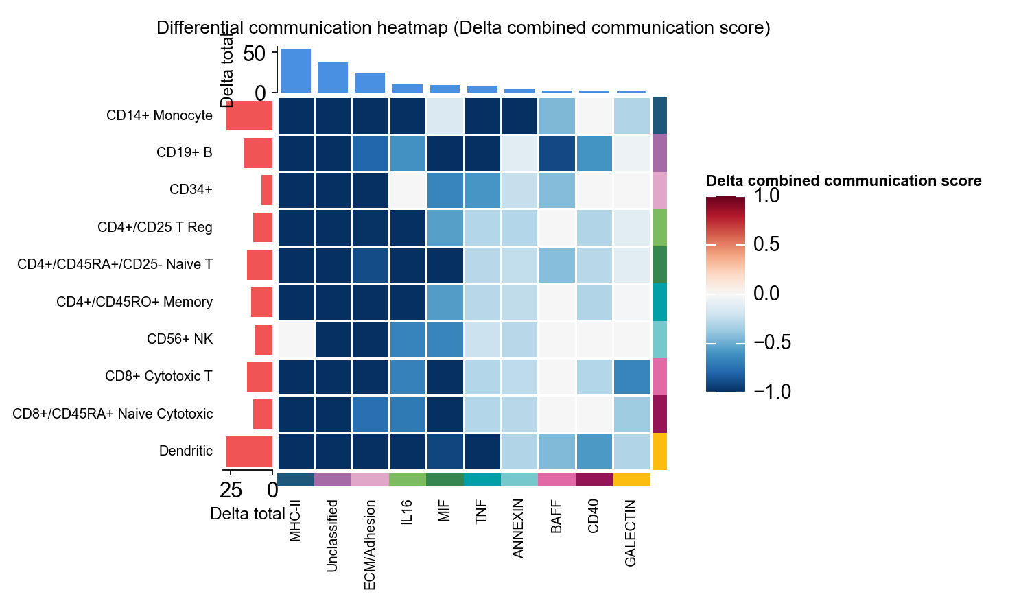
1.8 diff heatmap

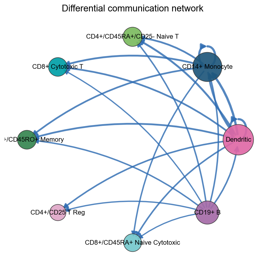
为了演示差异热图，这里直接基于 comm_adata 构造一个 synthetic comparison 对象。

fig, ax = ov.pl.ccc_heatmap(
    adata,
    comparison_adata=comparison_comm,
    plot_type='diff_heatmap',
    top_n=10,
    figsize=(5,5),
    show=False,
    show_col_names=True,
    show_row_names=True,
)

二、ov.pl.ccc_network_plot

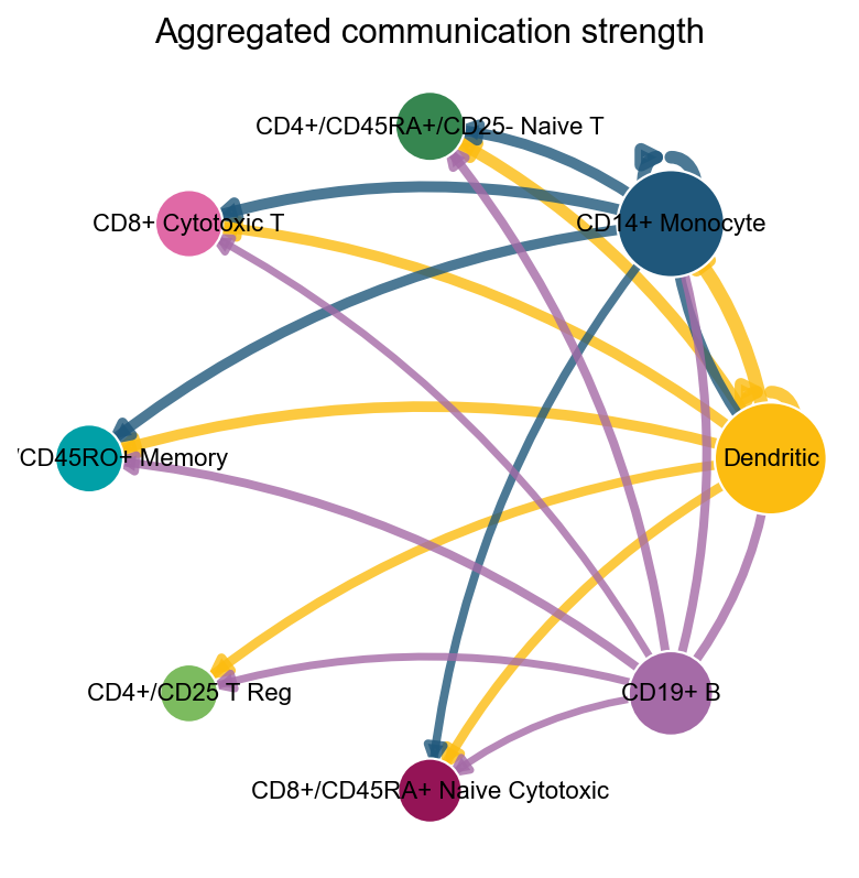
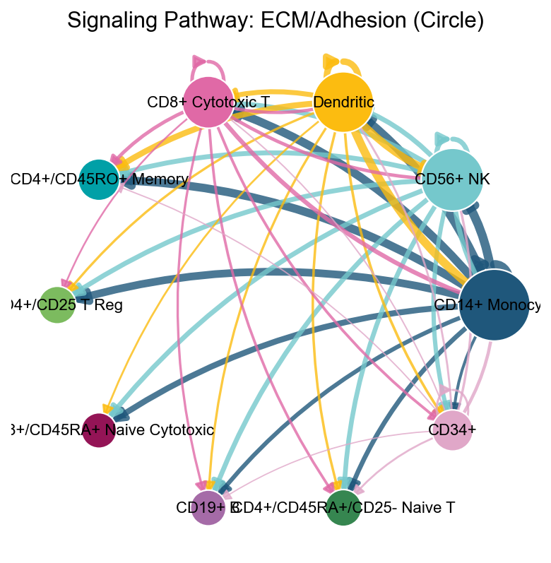
热图类视图适合看矩阵模式，网络类视图适合回答：

• 哪些细胞群是主 sender / 主 receiver

• 某个 pathway 的整体流向是什么

• 单个 ligand / receptor 的作用边界在哪里

fig, ax = ov.pl.ccc_network_plot(
    adata,
    plot_type='circle',
    palette=color_dict,
    title='Aggregated communication strength',
    figsize=(6, 6),
    show=False,
)

fig, ax = ov.pl.ccc_network_plot(
    adata,
    plot_type='pathway',
    signaling=['ECM/Adhesion'],
    palette=color_dict,
    top_n=50,
    figsize=(6, 6),
    show=False,
)

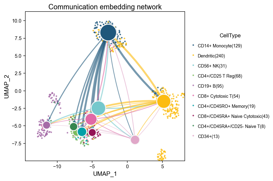
embedding_network 把细胞类型之间的通讯网络叠加到低维嵌入空间上。背景散点展示各细胞类型在整体转录组空间中的位置分布，较大的圆点表示聚合后的细胞类型节点，连线表示细胞类型之间的通讯方向和强度。这样可以同时观察“细胞在表达空间中的相对邻近关系”和“哪些细胞类型之间存在更强的通讯联系”，适合用来判断通讯是否主要发生在空间上接近或功能上相关的细胞群之间。

fig, ax = ov.pl.ccc_network_plot(
    adata,
    plot_type='embedding_network',
    signaling=['ECM/Adhesion'],
    node_positions=node_positions,
    embedding_points=embedding_points,
    palette=color_dict,
    top_n=50,
    figsize=(6, 5),
    show=False,
)

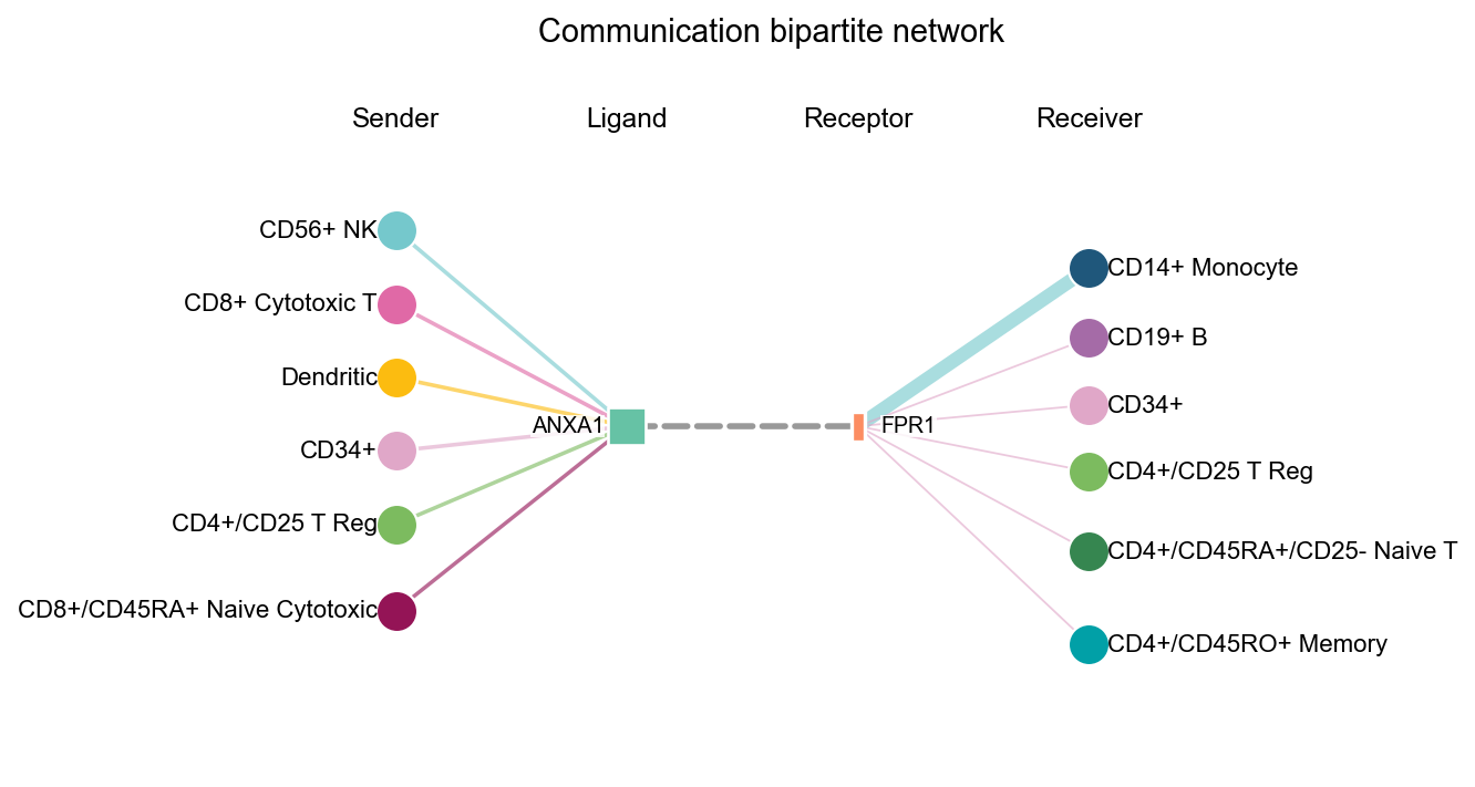
fig, ax = ov.pl.ccc_network_plot(
    comm_adata,
    plot_type='bipartite',
    ligand=focus_ligand,
    palette=color_dict,
    top_n=6,
    figsize=(6, 5),
    show=False,
)

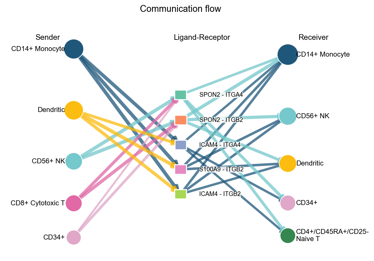
fig, ax = ov.pl.ccc_network_plot(
    adata,
    plot_type='arrow',
    display_by='interaction',
    signaling=['ECM/Adhesion'],
    palette=color_dict,
    top_n=5,
    figsize=(8, 6),
    show=False,
)

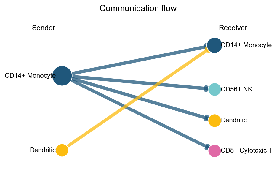
arrow、sigmoid支持设置display_by='aggregation'，这样图上只会保留Sender和Receiver互作关系对，此时top_n控制显示关系数量。

fig, ax = ov.pl.ccc_network_plot(
    adata,
    plot_type='arrow',
    display_by='aggregation',
    signaling=['ECM/Adhesion'],
    palette=color_dict,
    top_n=5,
    figsize=(6, 4),
    show=False,
)

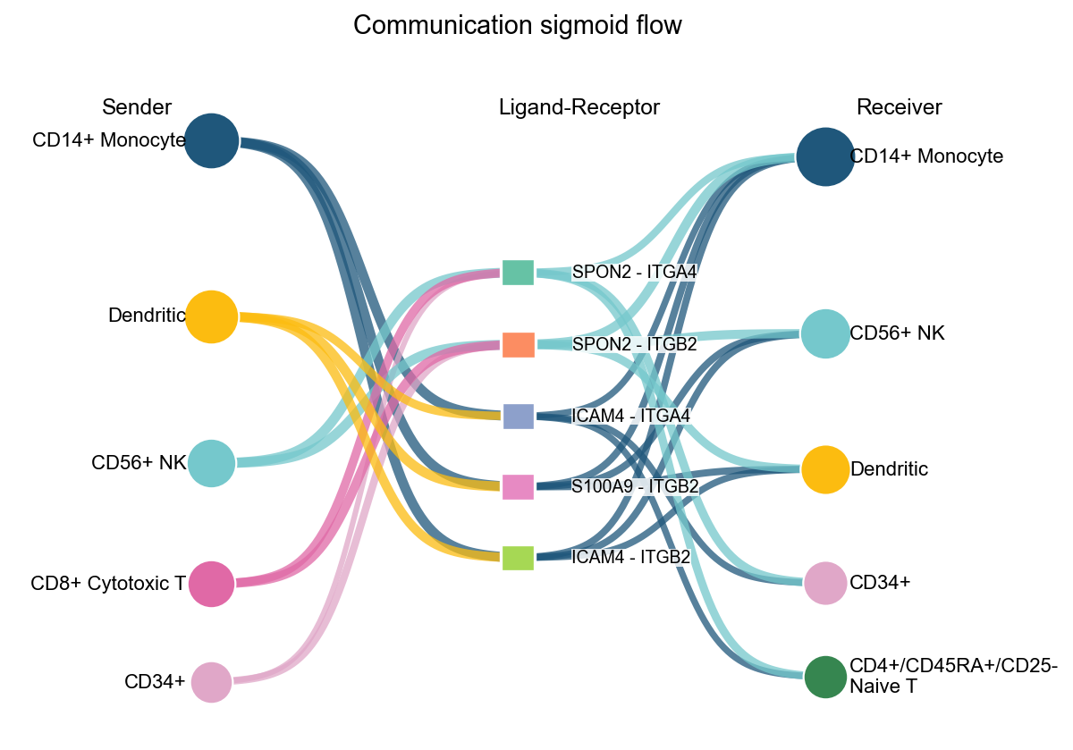
fig, ax = ov.pl.ccc_network_plot(
    adata,
    plot_type='sigmoid',
    display_by='interaction',
    signaling=['ECM/Adhesion'],
    palette=color_dict,
    top_n=5,
    figsize=(8, 6),
    show=False,
)

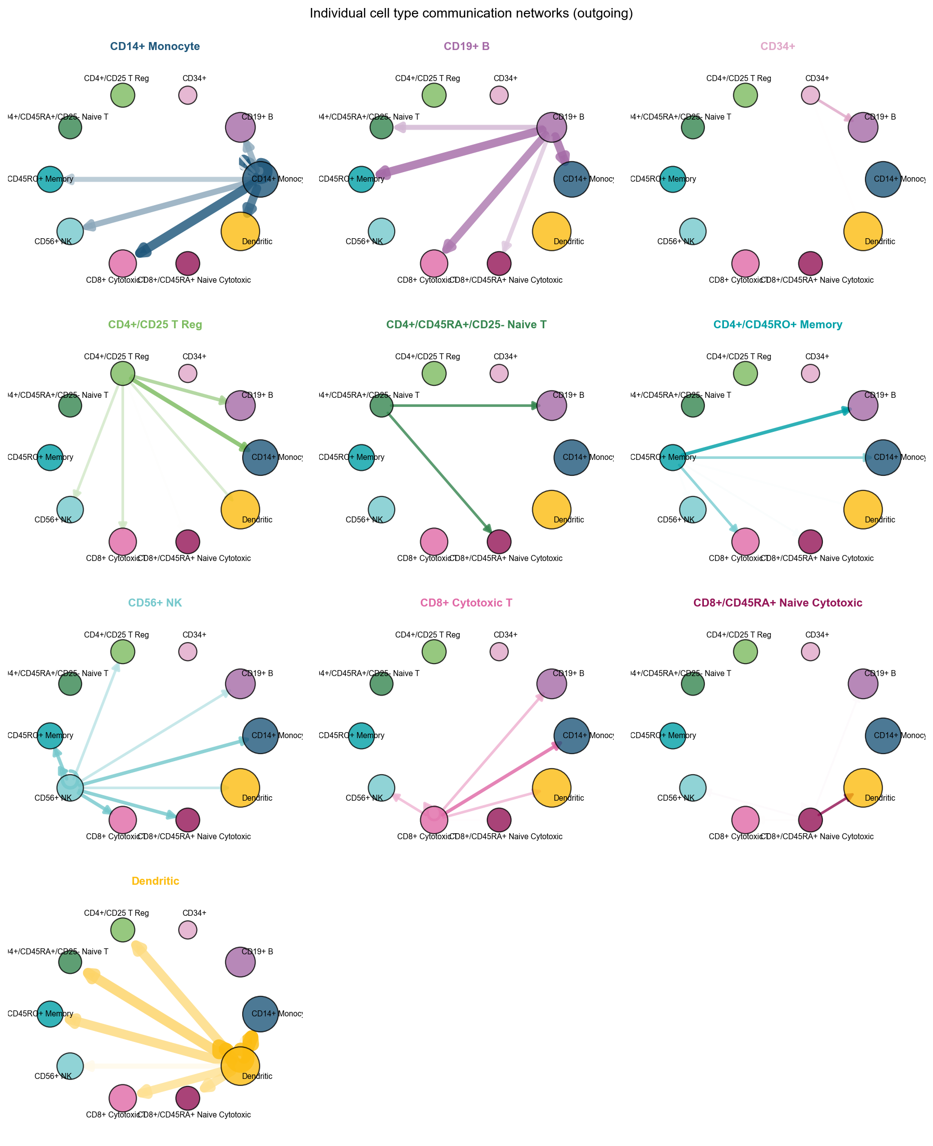
fig, ax = ov.pl.ccc_network_plot(
    adata,
    plot_type='individual_outgoing',
    figsize=(12, 15),
    ncols=3,
    show=False,
)

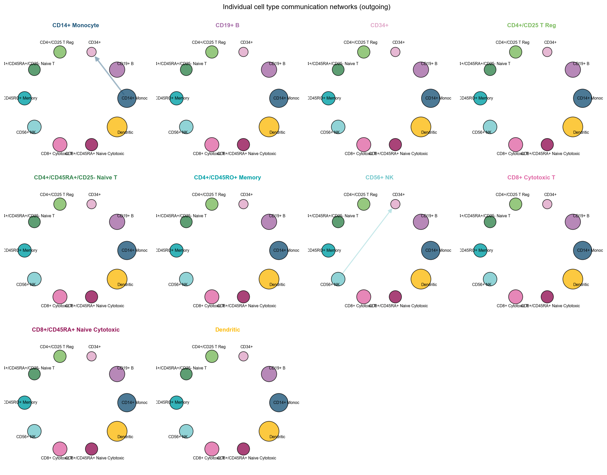
fig, ax = ov.pl.ccc_network_plot(
    adata,
    plot_type='individual_outgoing',
    receiver_use='CD34+',
    figsize=(15, 12),
    show=False,
)

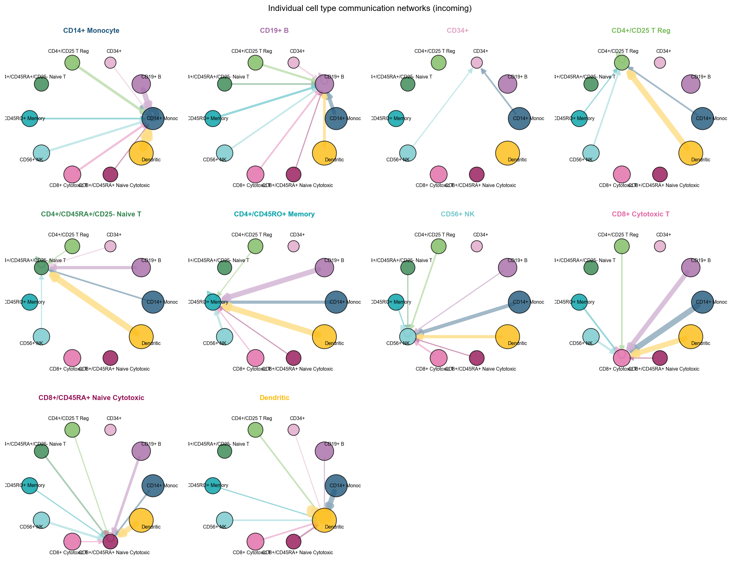
fig, ax = ov.pl.ccc_network_plot(
    adata,
    plot_type='individual_incoming',
    figsize=(15, 12),
    show=False,
)

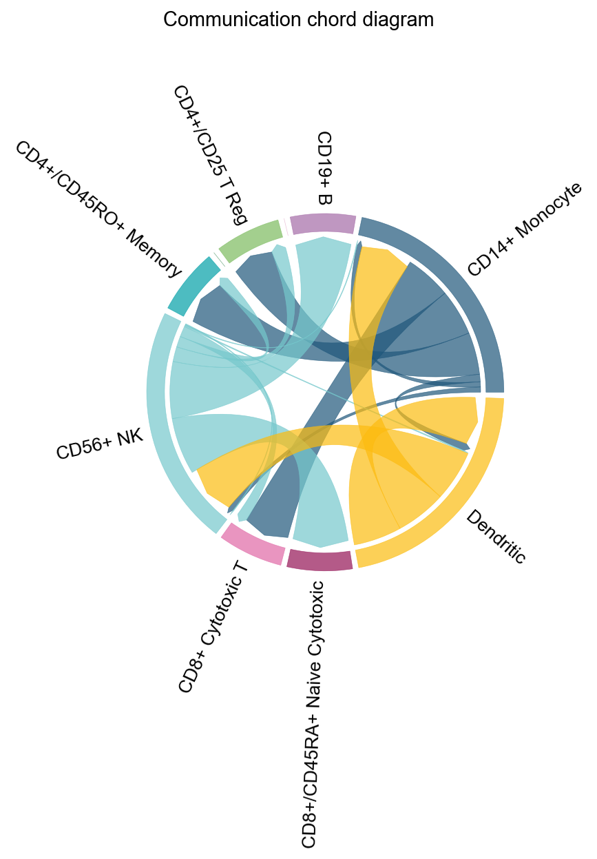
fig, ax = ov.pl.ccc_network_plot(
    adata,
    plot_type='chord',
    signaling=['ECM/Adhesion'],
    normalize_to_sender=True,
    figsize=(8, 8),
    show=False,
)

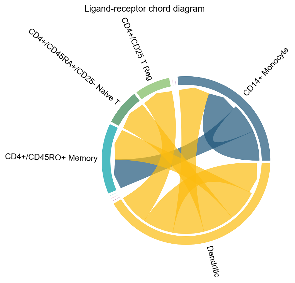
fig, ax = ov.pl.ccc_network_plot(
    adata,
    plot_type='lr_chord',
    pair_lr_use=focus_pair_lr,
    palette=color_dict,
    figsize=(6, 6),
    show=False,
)

fig, ax = ov.pl.ccc_network_plot(
    adata,
    comparison_adata=comparison_comm,
    plot_type='diff_network',
    top_n=20,
    show=False,
)

三、ov.pl.ccc_stat_plot

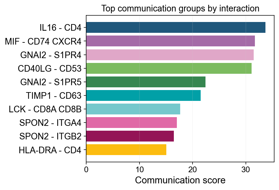
统计类图用于做排序、压缩和解释：

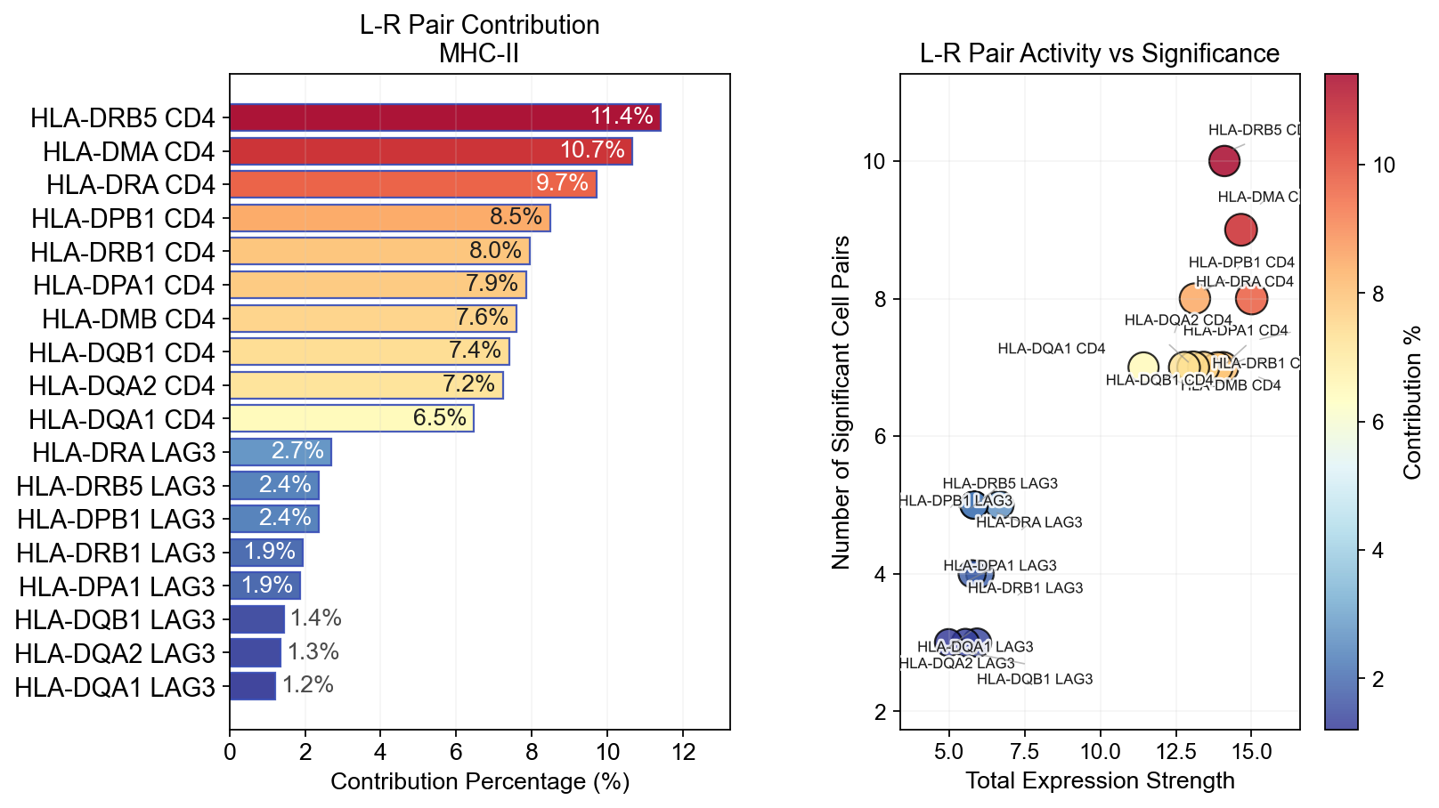
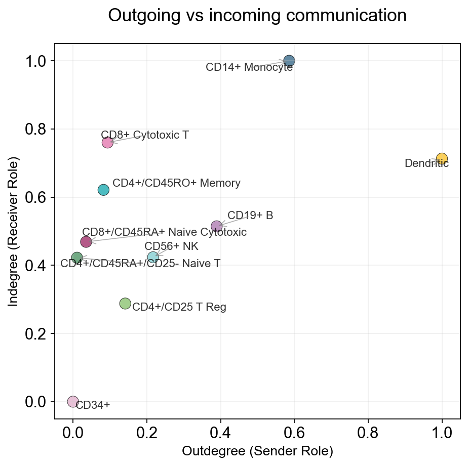
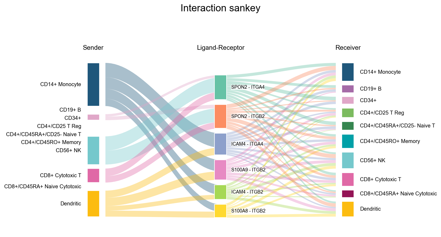
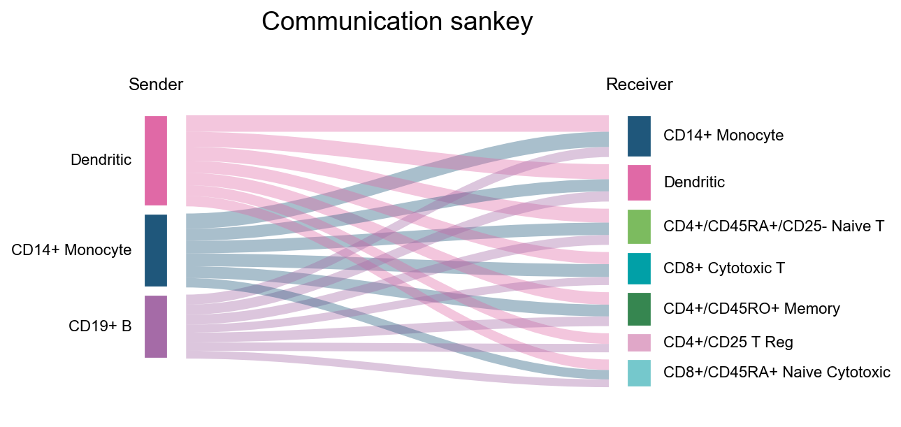
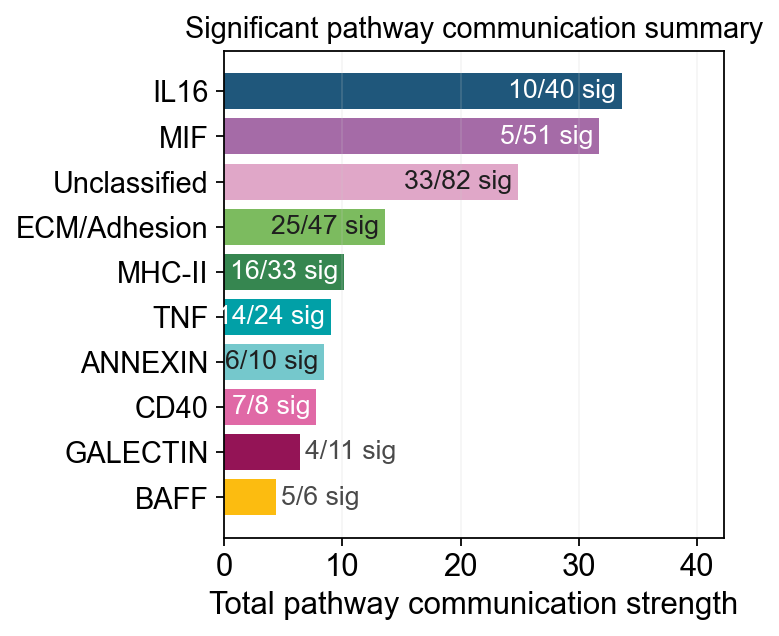
• bar：最紧凑的 interaction / pathway 排序

• scatter：看总体 communication 分布

• sankey：看 sender / receiver / interaction 的流向关系

• pathway_summary：看 pathway 级总强度与显著 pair 数

• lr_contribution：看某个 pathway 内部由哪些 ligand-receptor pair 构成

fig, ax = ov.pl.ccc_stat_plot(
    adata,
    plot_type='bar',
    display_by='interaction',
    score_key='specificity_rank',
    pvalue_key='specificity_rank',
    group_by='interaction',
    top_n=10,
    figsize=(5, 4),
    show=False,
)

fig, ax = ov.pl.ccc_stat_plot(
    adata,
    plot_type='scatter',
    figsize=(6, 6),
    show=False,
)

✅ Network centrality calculation completed (CellChat-style Importance values)
   - Signaling pathways used: All pathways
   - Weight mode: Weighted
   - Calculated metrics: outdegree, indegree, flow_betweenness, information, overall
   - All centrality scores normalized to 0-1 range (Importance values)

fig, ax = ov.pl.ccc_stat_plot(
    adata,
    plot_type='sankey',
    display_by='interaction',
    signaling=['ECM/Adhesion'],
    figsize=(8, 6),
    show=False,
)

fig, ax = ov.pl.ccc_stat_plot(
    adata,
    plot_type='sankey',
    display_by='aggregation',
    figsize=(6, 4),
    show=False,
)

fig, ax = ov.pl.ccc_stat_plot(
    adata,
    plot_type='pathway_summary',
    score_key='specificity_rank',
    pvalue_key='specificity_rank',
    classification_reference='cellchat',
    classification_fallback='family',
    top_n=10,
    pvalue_threshold=0.05,
    min_expression=0.0,
    strength_threshold=0.0,
    min_significant_pairs=1,
    figsize=(4, 4),
    verbose=True,
    show=False,
)

🔬 Calculating cell communication strength for 11 pathways...
   - Aggregation method: mean
   - Minimum expression threshold: 0.0
✅ Completed pathway communication strength calculation for 11 pathways
📊 Pathway significance analysis results:
   - Total pathways: 11
   - Significant pathways: 11
   - Strength threshold: 0.0
   - p-value threshold: 0.05

🏆 Top 10 pathways by total strength:
----------------------------------------------------------------------------------------------------
Pathway                        Total    Max     Mean    L-R  Active Sig  Rate   Status
----------------------------------------------------------------------------------------------------
IL16                           33.69    0.98    0.84    1    40     10   0.25   ***
MIF                            31.72    0.98    0.62    1    51     5    0.10   ***
Unclassified                   24.84    0.67    0.30    5    82     33   0.40   ***
ECM/Adhesion                   13.60    0.67    0.29    6    47     25   0.53   ***
MHC-II                         10.13    0.55    0.31    18   33     16   0.48   ***
TNF                            9.02     0.91    0.38    3    24     14   0.58   ***
ANNEXIN                        8.44     1.00    0.84    2    10     6    0.60   ***
CD40                           7.79     1.00    0.97    1    8      7    0.88   ***
GALECTIN                       6.39     1.00    0.58    1    11     4    0.36   ***
BAFF                           4.42     1.00    0.74    2    6      5    0.83   ***

fig, ax = ov.pl.ccc_stat_plot(
    adata,
    plot_type='lr_contribution',
    signaling=['MHC-II'],
    figsize=(10, 6),
    show=False,
)