单细胞空间转移张量#
空间转移张量(STT),一个使用信息论的方法…
import omicverse as ov
# 导入 OmicVerse.STT as st
import scvelo as scv
import scanpy as sc
ov.plot_set()
____            _     _    __
  / __ \____ ___  (_)___| |  / /__  _____________
 / / / / __ `__ \/ / ___/ | / / _ \/ ___/ ___/ _ \
/ /_/ / / / / / / / /__ | |/ /  __/ /  (__  )  __/
\____/_/ /_/ /_/_/\___/ |___/\___/_/  /____/\___/

Version: 1.5.10, Tutorials: https://omicverse.readthedocs.io/
预处理数据#
在本教程中,我们专注于演示和重现原始作者的结果…
adata = sc.read_h5ad('mouse_brain.h5ad')adata
AnnData object with n_obs × n_vars = 4628 × 117
    obs: 'n_counts', 'Region', 'Subclass', 'leiden', 'velocity_self_transition'
    var: 'GeneName', 'mean', 'std', 'velocity_gamma', 'velocity_qreg_ratio', 'velocity_r2', 'velocity_genes', 'highly_variable'
    uns: 'leiden', 'leiden_colors', 'neighbors', 'pca', 'umap', 'velocity_graph', 'velocity_graph_neg', 'velocity_params'
    obsm: 'X_pca', 'X_xy_loc', 'velocity_xy_loc', 'xy_loc'
    varm: 'PCs'
    layers: 'Ms', 'Mu', 'spliced', 'unspliced', 'variance_velocity', 'velocity'
    obsp: 'connectivities', 'distances'
Training STT modelHere, we used ov.space.STT 到 construct a STAGATE object 到 train 该 model. We need 到 set 该 following 参数 during initialisation:- spatial_loc: 该 nulling coordinates 对于 each 点位, 在 10x genomic 数据, are typically adata.obsm[‘spatial’], so 此 参数 is typically set 到 spatial, but 这里我们 store it 在 xy_loc.- region: 此 参数 is considered 到 be 该 region 的 该 attractor, which we would normally define using spatial annotations 或 cellular 注释 information.#
STT_obj=ov.space.STT(adata,spatial_loc='xy_loc',region='Region')
Note 那 we need 到 specify 该 number 的 potential attractors first when predicting attractors. 在 该 author’s original 教程 和 original paper, there is no clear definition 对于 该 specification 的 此 参数. After referring 到 该 author’s 教程, we use 该 calculated number 的 Leiden 的 adata_aggr 作为 a prediction 的 该 number 的 potential attractors.
STT_obj.stage_estimate()
computing PCA
    with n_comps=50
    finished (0:00:00)
computing neighbors
    using 'X_pca' with n_pcs = 50
    finished: added to `.uns['neighbors']`
    `.obsp['distances']`, distances for each pair of neighbors
    `.obsp['connectivities']`, weighted adjacency matrix (0:00:05)
running Leiden clustering
    finished: found 9 clusters and added
    'leiden', the cluster labels (adata.obs, categorical) (0:00:00)
...estimate stage: 9
该 authors noted 在 该 original 教程 那 a key 参数 called ‘spa_weight’ controls 该 relative weight 的 该 spatial location 相似度 内核.Other 参数 are further described 在 该 api 文档. Typically n_stage is 该 参数 we are interested 在 modifying
STT_obj.train(n_states = 9, n_iter = 15, weight_connectivities = 0.5, n_neighbors = 50,thresh_ms_gene = 0.2, spa_weight =0.3)
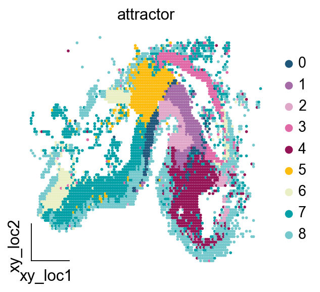
After 该 prediction is complete, 该 attractor is stored 在 adata.obs[‘attractor’]. 我们可以 use ov.pl.embedding 到 可视化 it.
ov.pl.embedding(adata, basis="xy_loc", color=["attractor"],frameon='small', palette=ov.pl.sc_color[11:])
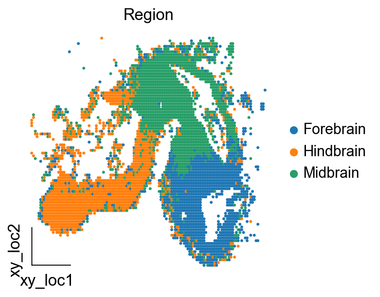
ov.pl.embedding(adata, basis="xy_loc", color=["Region"],frameon='small', )
Pathway analysisIn 该 original 教程, 该 author encapsulated 该 gseapy==1.0.4 version 对于 access enrichment. Note 那 该 use 的 此 函数 requires networking, which we have modified so 那 我们可以 enrich using 该 local pathway datasetWe can download 好的 access 数据 directly 在 enrichr, such 作为 该 KEGG_2019_mouse used 在 此 study.https://maayanlab.cloud/Enrichr/geneSetLibrary?mode=text&libraryName=KEGG_2019_Mouse#
pathway_dict=ov.utils.geneset_prepare('genesets/KEGG_2019_Mouse.txt',organism='Mouse')
STT_obj.compute_pathway(pathway_dict)
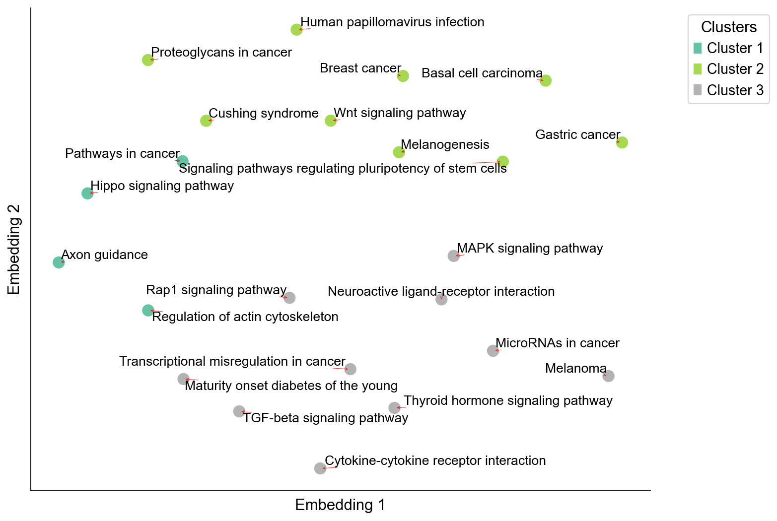
After running 该 函数, 我们可以 use 该 plot_pathway 函数 到 可视化 该 similairty between pathway dynamics 在 该 低 dimensional 嵌入.
fig = STT_obj.plot_pathway(figsize = (10,8),size = 100,fontsize = 12)for ax in fig.axes: ax.set_xlabel('Embedding 1', fontsize=20) # Adjust font 大小 作为 needed ax.set_ylabel('嵌入 2', fontsize=20) # Adjust font 大小 作为 neededfig.显示()
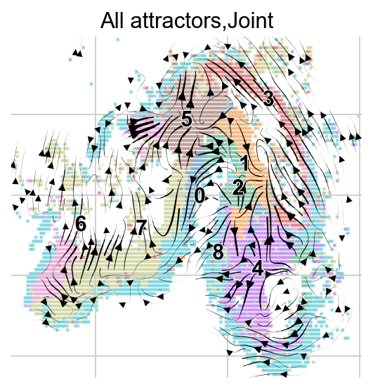
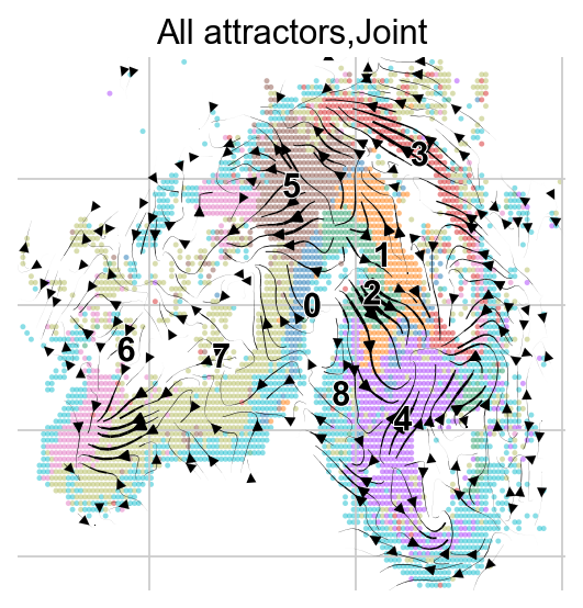
如果 we are interested 在 该 specific pathways, 我们可以 use 该 plot_tensor_pathway 函数 到 可视化 该 streamlines.
import matplotlib.pyplot as pltfig, ax = plt.subplots(1, 1, figsize=(4, 4))STT_obj.plot_tensor_pathway(pathway_name = 'Wnt signaling pathway',basis = 'xy_loc', ax=ax)
check that the input includes aggregated object
computing velocity graph (using 12/12 cores)
finished (0:00:02) --> added
    'vj_graph', sparse matrix with cosine correlations (adata.uns)
computing velocity embedding
    finished (0:00:00) --> added
    'vj_xy_loc', embedded velocity vectors (adata.obsm)
<AxesSubplot: title={'center': 'All attractors,Joint'}>
fig, ax = plt.subplots(1, 1, figsize=(4, 4))STT_obj.plot_tensor_pathway( 'TGF-beta signaling pathway',basis = 'xy_loc', ax=ax)
check that the input includes aggregated object
computing velocity graph (using 12/12 cores)
finished (0:00:02) --> added
    'vj_graph', sparse matrix with cosine correlations (adata.uns)
computing velocity embedding
    finished (0:00:00) --> added
    'vj_xy_loc', embedded velocity vectors (adata.obsm)
<AxesSubplot: title={'center': 'All attractors,Joint'}>
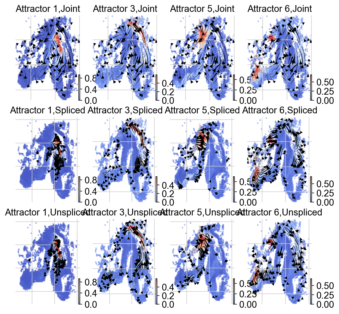
Tensor analysisIn 该 author’s original paper, a very interesting concept is mentioned, attractor-averaged 和 attractor-specific tensors.我们可以 分析 该 Joint Tensor 和 thus study 该 steady state processes 的 different attractors. 如果 该 streamlines are passing through 该 attractor then 该 attractor is 在 a steady state, 如果 该 streamlines are emanating/converging 从 该 attractor then 该 attractor is 在 a dynamic state.在 addition 到 此, 该 Unspliced Tensor also reflects 该 strength 作为 well 作为 该 大小 的 该 attraction.#
STT_obj.plot_tensor(list_attractor = [1,3,5,6], filter_cells = True, member_thresh = 0.1, density = 1)
check that the input includes aggregated object
computing velocity graph (using 12/12 cores)
finished (0:00:09) --> added
    'vj_graph', sparse matrix with cosine correlations (adata.uns)
computing velocity embedding
    finished (0:00:00) --> added
    'vj_xy_loc', embedded velocity vectors (adata.obsm)
check that the input includes aggregated object
computing velocity graph (using 12/12 cores)
finished (0:00:03) --> added
    'vj_graph', sparse matrix with cosine correlations (adata.uns)
computing velocity embedding
    finished (0:00:00) --> added
    'vj_xy_loc', embedded velocity vectors (adata.obsm)
check that the input includes aggregated object
computing velocity graph (using 12/12 cores)
finished (0:00:03) --> added
    'vj_graph', sparse matrix with cosine correlations (adata.uns)
computing velocity embedding
    finished (0:00:00) --> added
    'vj_xy_loc', embedded velocity vectors (adata.obsm)
check that the input includes aggregated object
computing velocity graph (using 12/12 cores)
finished (0:00:03) --> added
    'vj_graph', sparse matrix with cosine correlations (adata.uns)
computing velocity embedding
    finished (0:00:00) --> added
    'vj_xy_loc', embedded velocity vectors (adata.obsm)
computing velocity graph (using 12/12 cores)
finished (0:00:01) --> added
    'vs_graph', sparse matrix with cosine correlations (adata.uns)
computing velocity embedding
    finished (0:00:00) --> added
    'vs_xy_loc_aggr', embedded velocity vectors (adata.obsm)
computing velocity graph (using 12/12 cores)
finished (0:00:01) --> added
    'vs_graph', sparse matrix with cosine correlations (adata.uns)
computing velocity embedding
    finished (0:00:00) --> added
    'vs_xy_loc_aggr', embedded velocity vectors (adata.obsm)
computing velocity graph (using 12/12 cores)
finished (0:00:01) --> added
    'vs_graph', sparse matrix with cosine correlations (adata.uns)
computing velocity embedding
    finished (0:00:00) --> added
    'vs_xy_loc_aggr', embedded velocity vectors (adata.obsm)
computing velocity graph (using 12/12 cores)
finished (0:00:01) --> added
    'vs_graph', sparse matrix with cosine correlations (adata.uns)
computing velocity embedding
    finished (0:00:00) --> added
    'vs_xy_loc_aggr', embedded velocity vectors (adata.obsm)
computing velocity graph (using 12/12 cores)
finished (0:00:01) --> added
    'vu_graph', sparse matrix with cosine correlations (adata.uns)
computing velocity embedding
    finished (0:00:00) --> added
    'vu_xy_loc_aggr', embedded velocity vectors (adata.obsm)
computing velocity graph (using 12/12 cores)
finished (0:00:01) --> added
    'vu_graph', sparse matrix with cosine correlations (adata.uns)
computing velocity embedding
    finished (0:00:00) --> added
    'vu_xy_loc_aggr', embedded velocity vectors (adata.obsm)
computing velocity graph (using 12/12 cores)
finished (0:00:01) --> added
    'vu_graph', sparse matrix with cosine correlations (adata.uns)
computing velocity embedding
    finished (0:00:00) --> added
    'vu_xy_loc_aggr', embedded velocity vectors (adata.obsm)
computing velocity graph (using 12/12 cores)
finished (0:00:01) --> added
    'vu_graph', sparse matrix with cosine correlations (adata.uns)
computing velocity embedding
    finished (0:00:00) --> added
    'vu_xy_loc_aggr', embedded velocity vectors (adata.obsm)
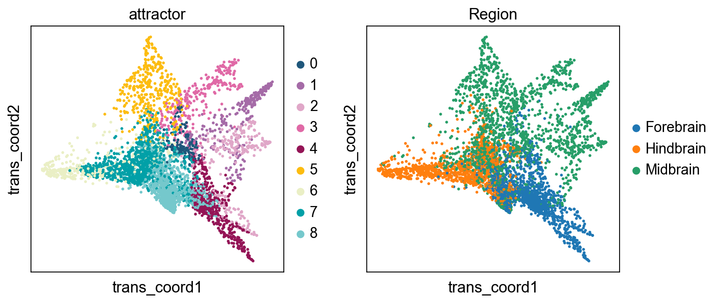
Landscape analysisEach attractor corresponds 到 a spatial steady state, then 我们可以 use contour plots 到 visualise 此 steady state 和 use CellRank’s 相关性 函数 到 infer state transitions between different attractors.#
STT_obj.construct_landscape(coord_key = 'X_xy_loc')
sc.pl.embedding(adata, color = ['attractor', 'Region'],basis= 'trans_coord')
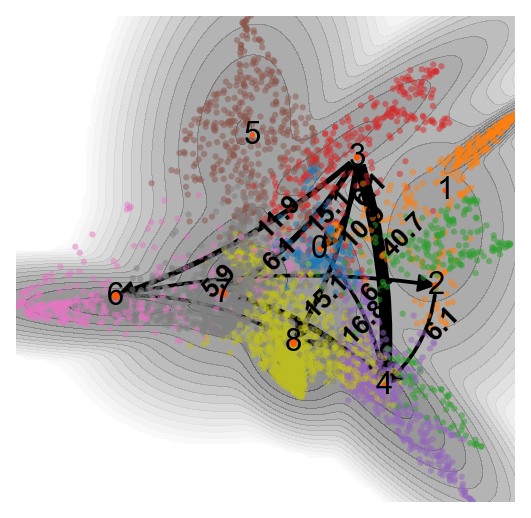
方法 到 infer 该 lineage, either ‘MPFT’(maxium 概率 flow tree, global) 或 ‘MPPT’(most probable 路径 tree, local)
STT_obj.infer_lineage(si=3,sf=4, method = 'MPPT',flux_fraction=0.8,color_palette_name = 'tab10',size_point = 8, size_text=12)
<AxesSubplot: >
该 Sankey 绘制 displaying 该 relation between STT attractors (left) 和 spatial region annotations (right). 该 width 的 links indicates 该 number 的 cells 那 share 该 connected attractor 标签 和 region 注释 标签 simultaneously
fig = STT_obj.plot_sankey(adata.obs['attractor'].tolist(),adata.obs['Region'].tolist())
Saving 和 Loading DataWe need 到 保存 该 数据 after 该 calculation is complete, 和 we provide 该 加载 函数 到 加载 it directly 在 该 next analysis 不使用 having 到 re-分析 it.#
# del adata.uns['r2_keep_train']#del adata.uns['r2_keep_test']#del adata.uns['内核']#del adata.uns['kernel_connectivities']STT_obj.adata.写入('数据/mouse_brain_adata.H5AD')STT_obj.adata_aggr.写入('数据/mouse_brain_adata_aggr.H5AD')
adata=ov.read('data/mouse_brain_adata.h5ad')adata_aggr=ov.read('data/mouse_brain_adata_aggr.h5ad')
STT_obj=ov.space.STT(adata,spatial_loc='xy_loc',region='Region')STT_obj.load(adata,adata_aggr)
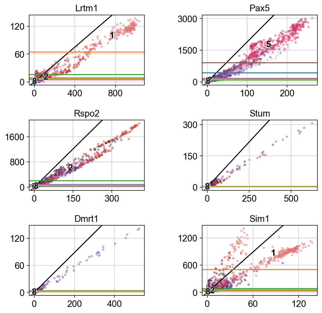
基因 DynamicThe 基因 使用 高 multistability scores possess varying 表达 levels 在 both unspliced 和 spliced 计数 within various attractors, 和 显示 a gradual change during stage transitions. 这些 基因 were stored 在 adata.var['r2_test']#
adata.var['r2_test'].sort_values(ascending=False)
Lrtm1     0.643272
Pax5      0.611002
Rspo2     0.596486
Stum      0.595376
Dmrt1     0.595088
            ...
Irx1     -0.337963
Bambi    -0.361296
Pou3f1   -0.367426
Fzd10    -0.379495
Ostm1    -0.988888
Name: r2_test, Length: 117, dtype: float64
STT_obj.plot_top_genes(top_genes = 6, ncols = 2, figsize = (8,8),)
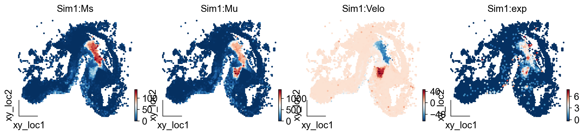
We analysed 该 attractor 1-related 基因 Sim1, 和 we found 那 在 该 unspliced Mu 矩阵 (smooth unspliced), Sim1 is expressed 低 在 attractor 1; 在 该 spliced 矩阵 Ms, Sim1 is expressed 高 在 attractor 1. It indicates 那 there is a dynamic tendency 的 Sim1 基因 在 attractor 1, i.e., 该 direction 的 Sim1 表达 is flowing towards attractor 1.Velo analyses can also illustrate 此, although Sim1 表达 is not highest 在 attractor 1.
import matplotlib.pyplot as pltfig, axes = plt.subplots(1, 4, figsize=(12, 3))ov.pl.embedding(adata, basis="xy_loc", color=["Sim1"],frameon='small', title='Sim1:Ms',show=False, layer='Ms',cmap='RdBu_r',ax=axes[0] )ov.pl.embedding(adata, basis="xy_loc", color=["Sim1"],frameon='small', title='Sim1:Mu',show=False, layer='Mu',cmap='RdBu_r',ax=axes[1] )ov.pl.embedding(adata, basis="xy_loc", color=["Sim1"],frameon='small', title='Sim1:Velo',show=False, layer='velo',cmap='RdBu_r',ax=axes[2] )ov.pl.embedding(adata, basis="xy_loc", color=["Sim1"],frameon='small', title='Sim1:exp',show=False, # layer='Mu', cmap='RdBu_r',ax=轴[3] )plt.tight_layout()