单细胞空间对齐工具

SLAT（空间链接对齐工具），一个基于图的算法…

# 导入 scSLAT
from omicverse.external.scSLAT.model import load_anndatas, Cal_Spatial_Net, run_SLAT

____            _     _    __                  
  / __ \____ ___  (_)___| |  / /__  _____________ 
 / / / / __ `__ \/ / ___/ | / / _ \/ ___/ ___/ _ \ 
/ /_/ / / / / / / / /__ | |/ /  __/ /  (__  )  __/ 
\____/_/ /_/ /_/_/\___/ |___/\___/_/  /____/\___/                                              

Version: 1.6.0, Tutorials: https://omicverse.readthedocs.io/

# 导入 scSLATfrom OmicVerse.external.scSLAT.model 导入 load_anndatas, Cal_Spatial_Net, run_SLAT, scanpy_workflow, spatial_matchfrom OmicVerse.external.scSLAT.viz 导入 match_3D_multi, hist, Sankey, match_3D_celltype, Sankey,Sankey_multi,build_3Dfrom OmicVerse.external.scSLAT.metrics 导入 region_statistics

预处理 Dataadata1.H5AD: E11.5 mouse embryo 数据集, download 从 hereadata2.H5AD: E12.5 mouse embryo 数据集, download 从 here

adata1 = sc.read_h5ad('data/E115_Stereo.h5ad')adata2 = sc.read_h5ad('data/E125_Stereo.h5ad')

adata1.obs['week']='E11.5'adata2.obs['week']='E12.5'

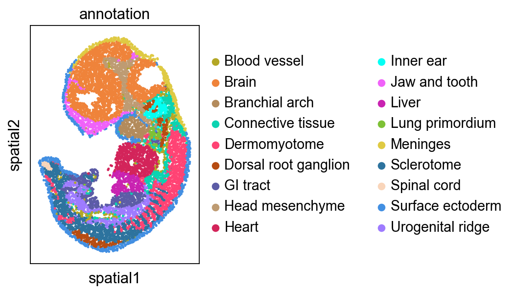
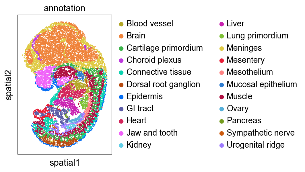
sc.pl.spatial(adata1, color='annotation', spot_size=3)sc.pl.spatial(adata2, color='annotation', spot_size=3)

Run SLATThen we run SLAT 作为 usual

Cal_Spatial_Net(adata1, k_cutoff=20, model='KNN')Cal_Spatial_Net(adata2, k_cutoff=20, model='KNN')edges, features = load_anndatas([adata1, adata2], feature='DPCA', check_order=False)

Calculating spatial neighbor graph ...
The graph contains 218282 edges, 10000 cells.
21.8282 neighbors per cell on average.
Calculating spatial neighbor graph ...
The graph contains 219259 edges, 10001 cells.
21.923707629237075 neighbors per cell on average.
Use DPCA feature to format graph
If you pass `n_top_genes`, all cutoffs are ignored.
extracting highly variable genes
--> added
    'highly_variable', boolean vector (adata.var)
    'highly_variable_rank', float vector (adata.var)
    'means', float vector (adata.var)
    'variances', float vector (adata.var)
    'variances_norm', float vector (adata.var)
normalizing counts per cell
    finished (0:00:00)
... as `zero_center=True`, sparse input is densified and may lead to large memory consumption
... as `zero_center=True`, sparse input is densified and may lead to large memory consumption
Warning! Dual PCA is using GPU, which may lead to OUT OF GPU MEMORY in big dataset!

embd0, embd1, time = run_SLAT(features, edges, LGCN_layer=5)

Choose GPU:0 as device
Running
---------- epochs: 1 ----------
---------- epochs: 2 ----------
---------- epochs: 3 ----------
---------- epochs: 4 ----------
---------- epochs: 5 ----------
---------- epochs: 6 ----------
Training model time: 1.21

best, index, distance = spatial_match([embd0, embd1], reorder=False, adatas=[adata1,adata2])

matching = np.array([range(index.shape[0]), best])best_match = distance[:,0]region_statistics(best_match, start=0.5, number_of_interval=10)

0.500~0.550         5          0.050%
0.550~0.600        48          0.480%
0.600~0.650       162          1.620%
0.650~0.700       425          4.250%
0.700~0.750      1004         10.039%
0.750~0.800      1578         15.778%
0.800~0.850      1900         18.998%
0.850~0.900      1701         17.008%
0.900~0.950      2141         21.408%
0.950~1.000      1036         10.359%

可视化 的 alignment

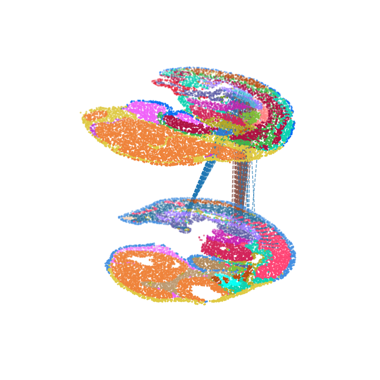
import matplotlib.pyplot as pltmatching_list=[matching]model = build_3D([adata1,adata2], matching_list,subsample_size=300, )ax=model.draw_3D(hide_axis=True, line_color='# c2c2c2', height=1, 大小=[6,6], line_width=1)

Mapping 0th layer

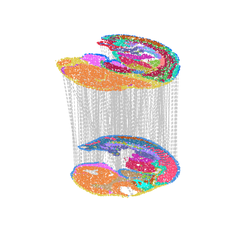
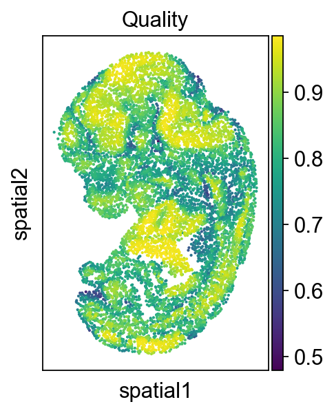
Then we check 该 alignment 质量 的 该 whole slide

adata2.obs['low_quality_index']= best_matchadata2.obs['low_quality_index'] = adata2.obs['low_quality_index'].astype(float)

adata2.obsm['spatial']

array([[-118.07557033,  391.48711306],
       [ -80.27430014,  356.96083362],
       [-130.37495374,  164.18395609],
       ...,
       [ -91.13328399,  258.15252187],
       [   7.42631645,  302.86275741],
       [ -98.93455418,  344.64032554]])

sc.pl.spatial(adata2, color='low_quality_index', spot_size=3, title='Quality')

We use a Sankey diagram 到 显示 该 correspondence between 细胞类型 在 different stages 的 development

fig=Sankey_multi(adata_li=[adata1,adata2],             prefix_li=['E11.5','E12.5'],             matching_li=[matching],                clusters='annotation',filter_num=10,             node_opacity = 0.8,             link_opacity = 0.2,                layout=[800,500],           font_size=12,           font_color='Black',           save_name=None,           format='png',           width=1200,           height=1000,           return_fig=True)fig.show()

fig.write_html("slat_sankey.html")

Focus 在 developing KidneyWe highlighted 该 “Kidney” cells 在 E12.5 和 their aligned precursor cells 在 E11.5 在 alignment results. Consistent 使用 our biological priors, 该 precursors 的 该 kidney are 该 mesonephros 和 该 metanephrosThen we focus 在 another organ: ‘Ovary’, 和 found ovary only has single spatial origin. It is interesting 那 precursors 的 ovary are spatially close 到 该 mesonephros (see Kidney part), because mammalian ovary originates 从 该 regressed mesonephros.

color_dict1=dict(zip(adata1.obs['annotation'].cat.categories,                    adata1.uns['annotation_colors'].tolist()))adata1_df = pd.DataFrame({'index':range(embd0.shape[0]),                          'x': adata1.obsm['spatial'][:,0],                          'y': adata1.obsm['spatial'][:,1],                          'celltype':adata1.obs['annotation'],                         'color':adata1.obs['annotation'].map(color_dict1)                         }                        )color_dict2=dict(zip(adata2.obs['annotation'].cat.categories,                    adata2.uns['annotation_colors'].tolist()))adata2_df = pd.DataFrame({'index':range(embd1.shape[0]),                          'x': adata2.obsm['spatial'][:,0],                          'y': adata2.obsm['spatial'][:,1],                          'celltype':adata2.obs['annotation'],                         'color':adata2.obs['annotation'].map(color_dict2)                         }                        )

kidney_align = match_3D_celltype(adata1_df, adata2_df, matching, meta='celltype',                                  highlight_celltype = [['Urogenital ridge'],['Kidney','Ovary']],                                 subsample_size=10000, highlight_line = ['blue'], scale_coordinate = True )kidney_align.draw_3D(size= [6, 6], line_width =0.8, point_size=[0.6,0.6], hide_axis=True)

dataset1: 18 cell types; dataset2: 22 cell types; 
                    Total :29 celltypes; Overlap: 11 cell types 
                    Not overlap :[['Dermomyotome', 'Surface ectoderm', 'Sclerotome', 'Inner ear', 'Spinal cord', 'Head mesenchyme', 'Branchial arch', 'Sympathetic nerve', 'Ovary', 'Pancreas', 'Mucosal epithelium', 'Muscle', 'Mesentery', 'Choroid plexus', 'Kidney', 'Epidermis', 'Cartilage primordium', 'Mesothelium']]
Subsampled 10000 pairs from 10001

我们可以 获取 该 lineage 的 该 query’s cells 和 mappings using 该 following 函数

def cal_matching_cell(target_adata,query_adata,matching,query_cell,clusters='annotation',):    adata1_df = pd.DataFrame({'index':range(target_adata.shape[0]),                          'x': target_adata.obsm['spatial'][:,0],                          'y': target_adata.obsm['spatial'][:,1],                          'celltype':target_adata.obs[clusters]})    adata2_df = pd.DataFrame({'index':range(query_adata.shape[0]),                              'x': query_adata.obsm['spatial'][:,0],                              'y': query_adata.obsm['spatial'][:,1],                              'celltype':query_adata.obs[clusters]})    query_adata = target_adata[matching[1,adata2_df.loc[adata2_df.celltype==query_cell,'index'].values],:]    # adata2_df['target_celltype'] = adata1_df.iloc[matching[1,:],:]['celltype'].to_list()    #adata2_df['target_obs_names'] = adata1_df.iloc[matching[1,:],:].index.to_list()        #query_obs=adata2_df.loc[adata2_df['celltype']==query_cell,'target_obs_names'].tolist()    return query_adata

We find 那 maps mapped 在 3D also 显示 up well 在 2D

query_adata=cal_matching_cell(target_adata=adata1,                              query_adata=adata2,                              matching=matching,                              query_cell='Kidney',clusters='annotation')query_adata

View of AnnData object with n_obs × n_vars = 59 × 26854
    obs: 'n_genes_by_counts', 'log1p_n_genes_by_counts', 'total_counts', 'log1p_total_counts', 'annotation', 'Regulon - A1cf', 'kidney_c0', 'kidney_c1', 'kidney_c2', 'kidney_c3', 'kidney_anno', 'week'
    var: 'n_cells', 'n_cells_by_counts', 'mean_counts', 'log1p_mean_counts', 'pct_dropout_by_counts', 'total_counts'
    uns: 'Spatial_Net', 'annotation_colors', 'kidney_c0_colors', 'kidney_c1_colors', 'kidney_c2_colors', 'kidney_c3_colors', 'kidney_anno_colors'
    obsm: 'spatial'
    varm: 'PCs'

adata1.obs['kidney_anno']=''adata1.obs.loc[query_adata.obs.index,'kidney_anno']=query_adata.obs['annotation']

sc.pl.spatial(adata1, color='kidney_anno', spot_size=3,             palette=['# F5F5F5','#ff7f0e', 'green',])

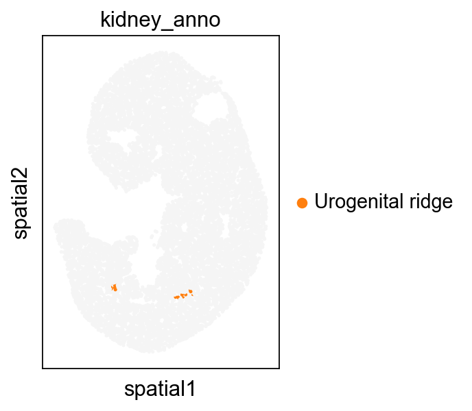
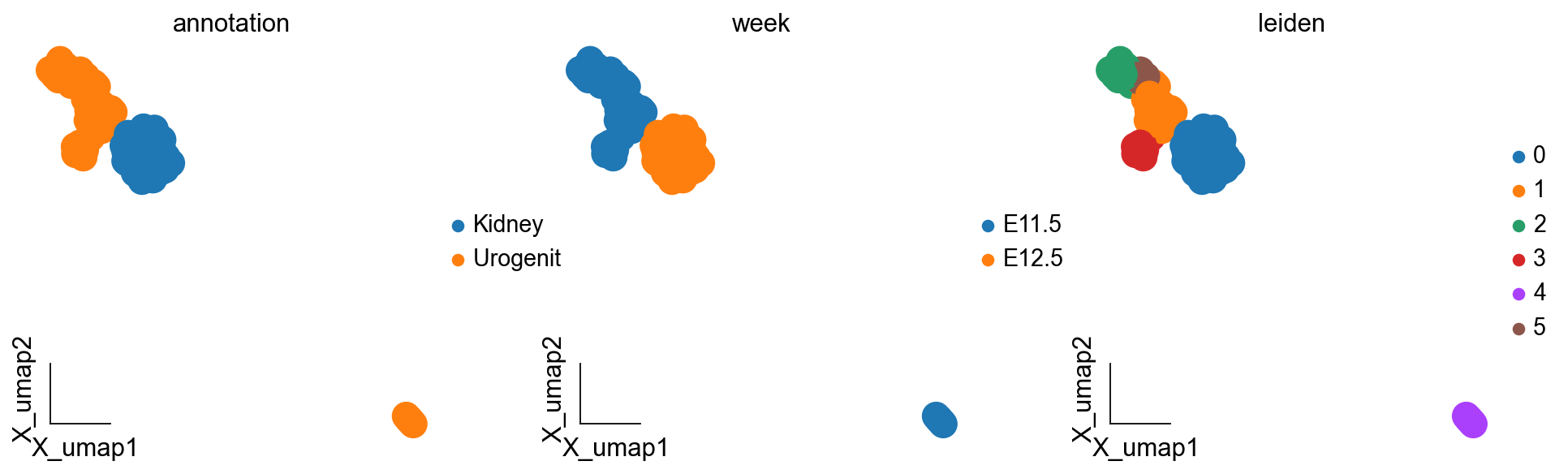
We are concerned 使用 Kidney lineage development, so we integrated 该 cells corresponding 到 该 Kidney lineage 在 该 two sections 的 E11 和 E12, 和 then we could use 该 方法 的 difference analysis 到 study 该 dynamic process 的 Kidney lineage development.

kidney_lineage_ad=sc.concat([query_adata,adata2[adata2.obs['annotation']=='Kidney']],merge='same')kidney_lineage_ad=ov.pp.preprocess(kidney_lineage_ad,mode='shiftlog|pearson',n_HVGs=3000,target_sum=1e4)kidney_lineage_ad.raw = kidney_lineage_adkidney_lineage_ad = kidney_lineage_ad[:, kidney_lineage_ad.var.highly_variable_features]ov.pp.scale(kidney_lineage_ad)ov.pp.pca(kidney_lineage_ad)ov.pp.neighbors(kidney_lineage_ad,use_rep='scaled|original|X_pca',metric="cosine")ov.utils.cluster(kidney_lineage_ad,method='leiden',resolution=1)ov.pp.umap(kidney_lineage_ad)

Begin robust gene identification
After filtration, 14823/26436 genes are kept. Among 14823 genes, 14823 genes are robust.
End of robust gene identification.
Begin size normalization: shiftlog and HVGs selection pearson
normalizing counts per cell The following highly-expressed genes are not considered during normalization factor computation:
[]
    finished (0:00:00)
extracting highly variable genes
--> added
    'highly_variable', boolean vector (adata.var)
    'highly_variable_rank', float vector (adata.var)
    'highly_variable_nbatches', int vector (adata.var)
    'highly_variable_intersection', boolean vector (adata.var)
    'means', float vector (adata.var)
    'variances', float vector (adata.var)
    'residual_variances', float vector (adata.var)
Time to analyze data in cpu: 0.07181000709533691 seconds.
End of size normalization: shiftlog and HVGs selection pearson
... as `zero_center=True`, sparse input is densified and may lead to large memory consumption
computing neighbors
    finished: added to `.uns['neighbors']`
    `.obsp['distances']`, distances for each pair of neighbors
    `.obsp['connectivities']`, weighted adjacency matrix (0:00:06)
running Leiden clustering
    finished: found 6 clusters and added
    'leiden', the cluster labels (adata.obs, categorical) (0:00:00)
computing UMAP
    finished: added
    'X_umap', UMAP coordinates (adata.obsm) (0:00:00)

ov.pl.embedding(kidney_lineage_ad,basis='X_umap',               color=['annotation','week','leiden'],               frameon='small')

# Nphs1 https://www.nature.com/articles/s41467-021-22266-1sc.pl.dotplot(kidney_lineage_ad,{'nephron progenitors':['Wnt9b','Osr1','Nphs1','Lhx1','Pax2','Pax8'],                         'metanephric':['Eya1','Shisa3','Foxc1'],                          'kidney':['Wt1','Wnt4','Nr2f2','Dach1','Cd44']} ,              'Leiden',dendrogram=False,colorbar_title='表达')

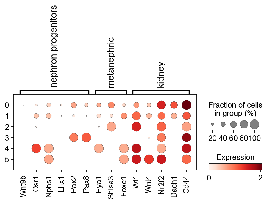
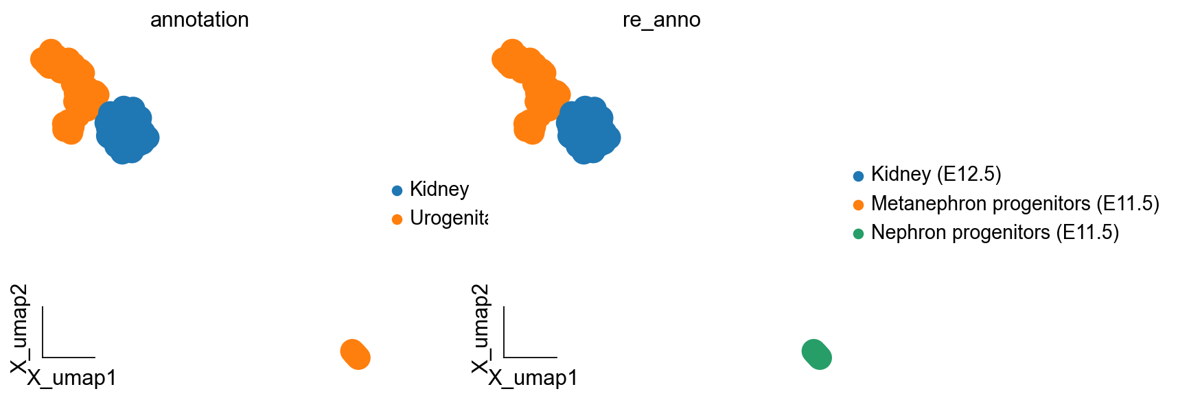
kidney_lineage_ad.obs['re_anno'] = 'Unknown'kidney_lineage_ad.obs.loc[kidney_lineage_ad.obs.leiden.isin(['4']),'re_anno'] = 'Nephron progenitors (E11.5)'kidney_lineage_ad.obs.loc[kidney_lineage_ad.obs.leiden.isin(['2','3','1','5']),'re_anno'] = 'Metanephron progenitors (E11.5)'kidney_lineage_ad.obs.loc[kidney_lineage_ad.obs.leiden=='0','re_anno'] = 'Kidney (E12.5)'

# kidney_all = kidney_all[kidney_all.obs.Leiden!='3',:]kidney_lineage_ad.obs.Leiden = list(kidney_lineage_ad.obs.Leiden)ov.pl.嵌入(kidney_lineage_ad,basis='X_umap',               颜色=['注释','re_anno'],               frameon='small')

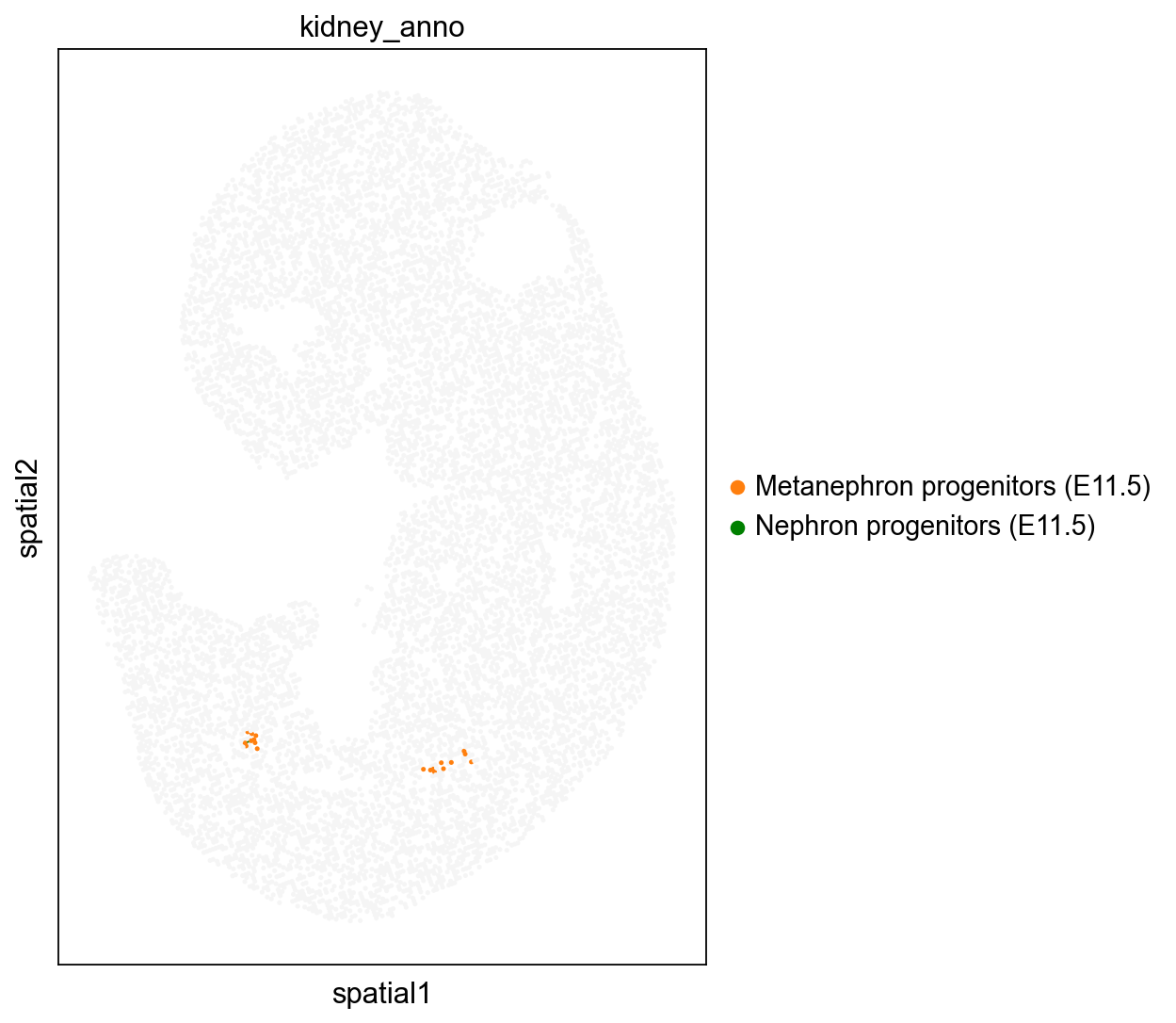
adata1.obs['kidney_anno']=''adata1.obs.loc[kidney_lineage_ad[kidney_lineage_ad.obs['week']=='E11.5'].obs.index,'kidney_anno']=kidney_lineage_ad[kidney_lineage_ad.obs['week']=='E11.5'].obs['re_anno']

import matplotlib.pyplot as pltfig, ax = plt.subplots(1, 1, figsize=(8, 8))sc.pl.spatial(adata1, color='kidney_anno', spot_size=1.5,             palette=['# F5F5F5','#ff7f0e', 'green',],显示=False,ax=ax)

[<AxesSubplot: title={'center': 'kidney_anno'}, xlabel='spatial1', ylabel='spatial2'>]

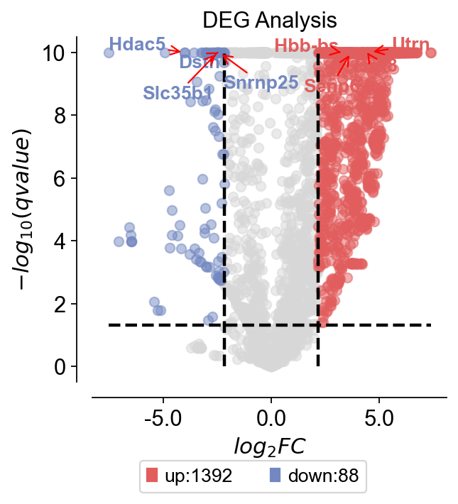
我们可以 also differentially 分析 Kidney’s developmental pedigree 到 find different 标记 基因, 和 我们可以 分析 transcription factors 和 thus find 该 regulatory units involved.

test_adata=kidney_lineage_addds=ov.bulk.pyDEG(test_adata.to_df(layer='lognorm').T)dds.drop_duplicates_index()print('... drop_duplicates_index success')treatment_groups=test_adata.obs[test_adata.obs['week']=='E12.5'].index.tolist()control_groups=test_adata.obs[test_adata.obs['week']=='E11.5'].index.tolist()result=dds.deg_analysis(treatment_groups,control_groups,method='ttest')# -1 means automatically calculatesdds.foldchange_set(fc_threshold=-1,                   pval_threshold=0.05,                   logp_max=10)

... drop_duplicates_index success
... Fold change threshold: 2.1686935424804688

dds.plot_volcano(title='DEG Analysis',figsize=(4,4),                 plot_genes_num=8,plot_genes_fontsize=12,)

<AxesSubplot: title={'center': 'DEG Analysis'}, xlabel='$log_{2}FC$', ylabel='$-log_{10}(qvalue)$'>

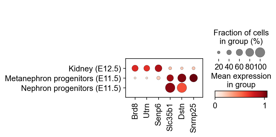
up_gene=dds.result.loc[dds.result['sig']=='up'].sort_values('qvalue')[:3].index.tolist()down_gene=dds.result.loc[dds.result['sig']=='down'].sort_values('qvalue')[:3].index.tolist()deg_gene=up_gene+down_gene

sc.pl.dotplot(kidney_lineage_ad,deg_gene,             groupby='re_anno')

在 addition 到 analysing directly using differential 表达, 我们可以 also look 对于 weekly 标记 基因 通过 considering weeks 作为 categories.

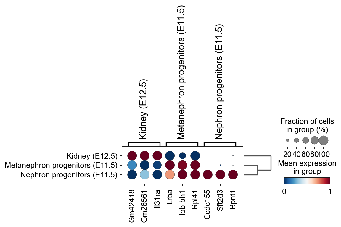
sc.tl.dendrogram(kidney_lineage_ad,'re_anno',use_rep='scaled|original|X_pca')sc.tl.rank_genes_groups(kidney_lineage_ad, 're_anno', use_rep='scaled|original|X_pca',                        method='t-test',use_raw=False,key_added='re_anno_ttest')sc.pl.rank_genes_groups_dotplot(kidney_lineage_ad,groupby='re_anno',                                cmap='RdBu_r',key='re_anno_ttest',                                standard_scale='var',n_genes=3)

Storing dendrogram info using `.uns['dendrogram_re_anno']`
ranking genes
    finished: added to `.uns['re_anno_ttest']`
    'names', sorted np.recarray to be indexed by group ids
    'scores', sorted np.recarray to be indexed by group ids
    'logfoldchanges', sorted np.recarray to be indexed by group ids
    'pvals', sorted np.recarray to be indexed by group ids
    'pvals_adj', sorted np.recarray to be indexed by group ids (0:00:00)