不使用参考 scRNA-seq 的空间反卷积#
这是一个关于在没有参考的情况下进行空间反卷积的教程。
import omicverse as ov
🔬 Starting plot initialization...
Using already downloaded Arial font from: /tmp/omicverse_arial.ttf
Registered as: Arial
🧬 Detecting GPU devices…
✅ NVIDIA CUDA GPUs detected: 1
    • [CUDA 0] NVIDIA H100 80GB HBM3
      Memory: 79.1 GB | Compute: 9.0

   ____            _     _    __
  / __ \____ ___  (_)___| |  / /__  _____________
 / / / / __ `__ \/ / ___/ | / / _ \/ ___/ ___/ _ \
/ /_/ / / / / / / / /__ | |/ /  __/ /  (__  )  __/
\____/_/ /_/ /_/_/\___/ |___/\___/_/  /____/\___/

🔖 Version: 1.7.9rc1   📚 Tutorials: https://omicverse.readthedocs.io/
✅ plot_set complete.
第1步:准备空间转录组学 (1 分钟)#
目的:加载 10x Visium (Space Ranger 输出) 或…
# 加载 scRNA-seq 参考
# 示例:人类淋巴结参考
adata_sc = ov.datasets.sc_ref_Lymph()
reading /scratch/users/steorra/analysis/omic_test/data/V1_Human_Lymph_Node/filtered_feature_bc_matrix.h5
 (0:00:00)
步骤 2: Prepare 该 基因 sig markergene_sig means 该 数据框 stored 该 标记 基因 在 each columns. 如果 you don’t have it, you can calculated it using ov.space.calculate_gene_signature#
# 加载 your scRNA-seq 参考# 示例: Human lymph node referenceadata_sc = ov.数据集.sc_ref_Lymph_Node()gene_sig=ov.space.calculate_gene_signature( adata_sc, clustertype='Subset', # 细胞类型 name rank=True, key='rank_genes_groups', foldchange=2, topgenenumber=20 )gene_sig.head()
🧬 Loading SC reference data for Lymph Node
🔍 Downloading data to ./data/sc_ref_Lymph_Node.h5ad
⚠️ File ./data/sc_ref_Lymph_Node.h5ad already exists
 Loading data from ./data/sc_ref_Lymph_Node.h5ad
✅ Successfully loaded: 73260 cells × 10237 genes
...get cell type marker
ranking genes
WARNING: It seems you use rank_genes_groups on the raw count data. Please logarithmize your data before calling rank_genes_groups.
    finished: added to `.uns['rank_genes_groups']`
    'names', sorted np.recarray to be indexed by group ids
    'scores', sorted np.recarray to be indexed by group ids
    'logfoldchanges', sorted np.recarray to be indexed by group ids
    'pvals', sorted np.recarray to be indexed by group ids
    'pvals_adj', sorted np.recarray to be indexed by group ids (0:01:00)
| B_Cycling | B_GC_DZ | B_GC_LZ | B_GC_prePB | B_IFN | B_activated | B_mem | B_naive | B_plasma | B_preGC | ... | T_CD4+_TfH | T_CD4+_TfH_GC | T_CD4+_naive | T_CD8+_CD161+ | T_CD8+_cytotoxic | T_CD8+_naive | T_TIM3+ | T_TfR | T_Treg | VSMC | |
|---|---|---|---|---|---|---|---|---|---|---|---|---|---|---|---|---|---|---|---|---|---|
| 0 | HMGN2 | CD79B | CD22 | BIK | HLA-DPA1 | HLA-DPA1 | HLA-DPA1 | HLA-DPA1 | SDF2L1 | HLA-DPA1 | ... | TRAC | TCF7 | RPS15A | ZFP36 | CD3E | NOSIP | TMSB4X | CD4 | TRAC | TAGLN |
| 1 | DEK | TCEA1 | PRPSAP2 | PRPSAP2 | ISG15 | HVCN1 | CD52 | HVCN1 | SSR3 | CD72 | ... | CD69 | SRGN | NOSIP | SRGN | CST7 | TCF7 | LCK | SRGN | SRGN | LGALS3 |
| 2 | HMGN1 | GAPDH | HMGN1 | VPREB3 | STAT1 | CD74 | SMIM14 | CD79B | PPIB | NME2 | ... | SRGN | PASK | TCF7 | RGCC | GZMK | RGCC | SRGN | CD3E | RGCC | CST3 |
| 3 | GAPDH | SUGCT | GAPDH | HMCES | CD74 | TCL1A | CD74 | CD72 | SEC61G | CD74 | ... | CD3E | ITM2A | RPS14 | CD8A | NKG7 | DNAJB1 | CD3E | ZAP70 | DNAJB1 | LAPTM4A |
| 4 | HMGB1 | EZR | CD74 | MEF2B | IFIT3 | HLA-DPB1 | VPREB3 | CD74 | HERPUD1 | HSP90AB1 | ... | SLC2A3 | CD3E | LEF1 | CCL5 | CTSW | LEF1 | CD27 | TCRA_VDJsum | FOXP3 | IGFBP5 |
5 rows × 34 columns
gene_sig.to_csv('data/gene_sig_Lymph_Node.csv')
gene_sig=ov.pd.read_csv('data/gene_sig_Lymph_Node.csv',index_col=0)gene_sig.head()
| B_Cycling | B_GC_DZ | B_GC_LZ | B_GC_prePB | B_IFN | B_activated | B_mem | B_naive | B_plasma | B_preGC | ... | T_CD4+_TfH | T_CD4+_TfH_GC | T_CD4+_naive | T_CD8+_CD161+ | T_CD8+_cytotoxic | T_CD8+_naive | T_TIM3+ | T_TfR | T_Treg | VSMC | |
|---|---|---|---|---|---|---|---|---|---|---|---|---|---|---|---|---|---|---|---|---|---|
| 0 | HMGN2 | CD79B | CD22 | BIK | HLA-DPA1 | HLA-DPA1 | HLA-DPA1 | HLA-DPA1 | SDF2L1 | HLA-DPA1 | ... | TRAC | TCF7 | RPS15A | ZFP36 | CD3E | NOSIP | TMSB4X | CD4 | TRAC | TAGLN |
| 1 | DEK | TCEA1 | PRPSAP2 | PRPSAP2 | ISG15 | HVCN1 | CD52 | HVCN1 | SSR3 | CD72 | ... | CD69 | SRGN | NOSIP | SRGN | CST7 | TCF7 | LCK | SRGN | SRGN | LGALS3 |
| 2 | HMGN1 | GAPDH | HMGN1 | VPREB3 | STAT1 | CD74 | SMIM14 | CD79B | PPIB | NME2 | ... | SRGN | PASK | TCF7 | RGCC | GZMK | RGCC | SRGN | CD3E | RGCC | CST3 |
| 3 | GAPDH | SUGCT | GAPDH | HMCES | CD74 | TCL1A | CD74 | CD72 | SEC61G | CD74 | ... | CD3E | ITM2A | RPS14 | CD8A | NKG7 | DNAJB1 | CD3E | ZAP70 | DNAJB1 | LAPTM4A |
| 4 | HMGB1 | EZR | CD74 | MEF2B | IFIT3 | HLA-DPB1 | VPREB3 | CD74 | HERPUD1 | HSP90AB1 | ... | SLC2A3 | CD3E | LEF1 | CCL5 | CTSW | LEF1 | CD27 | TCRA_VDJsum | FOXP3 | IGFBP5 |
5 rows × 34 columns
步骤 3: 解卷积 使用 starfyshWe perform n_repeat random restarts 和 选择 该 best model 使用 lowest loss 对于 参数 c (inferred 细胞类型 proportions):STARFYSH is integrated into 该 omicverse.space.Deconvolution 类. Simply set method='starfysh'.### Key 参数- n_repeats: Number 的 restart 到 run STARFYSH.- epochs: number 的 iterations- device: 该 trainning device#
# Initialize 该 解卷积 objectdecov_obj = ov.space.解卷积( adata_sp=adata_sp)
decov_obj.preprocess_sp( mode='pearsonr',n_svgs=3000,target_sum=1e4, subset_genes=False,)
🔍 [2026-01-11 23:07:13] Running preprocessing in 'cpu' mode...
Begin robust gene identification
    After filtration, 25187/36601 genes are kept.
    Among 25187 genes, 22411 genes are robust.
✅ Robust gene identification completed successfully.
Begin size normalization: shiftlog and HVGs selection pearson

🔍 Count Normalization:
   Target sum: 10000.0
   Exclude highly expressed: True
   Max fraction threshold: 0.2
   ⚠️ Excluding 1 highly-expressed genes from normalization computation
   Excluded genes: ['IGKC']

✅ Count Normalization Completed Successfully!
   ✓ Processed: 4,035 cells × 22,411 genes
   ✓ Runtime: 0.47s

🔍 Highly Variable Genes Selection (Experimental):
   Method: pearson_residuals
   Target genes: 3,000
   Theta (overdispersion): 100

✅ Experimental HVG Selection Completed Successfully!
   ✓ Selected: 3,000 highly variable genes out of 22,411 total (13.4%)
   ✓ Results added to AnnData object:
     • 'highly_variable': Boolean vector (adata.var)
     • 'highly_variable_rank': Float vector (adata.var)
     • 'highly_variable_nbatches': Int vector (adata.var)
     • 'highly_variable_intersection': Boolean vector (adata.var)
     • 'means': Float vector (adata.var)
     • 'variances': Float vector (adata.var)
     • 'residual_variances': Float vector (adata.var)
    Time to analyze data in cpu: 3.05 seconds.
computing PCA
    with n_comps=50
    finished (0:00:01)
✅ Preprocessing completed successfully.
    Added:
        'highly_variable_features', boolean vector (adata.var)
        'means', float vector (adata.var)
        'variances', float vector (adata.var)
        'residual_variances', float vector (adata.var)
        'counts', raw counts layer (adata.layers)
    End of size normalization: shiftlog and HVGs selection pearson
✓ spatial transcriptomics data is preprocessed
%time# Run FlashDeconv deconvolutiondecov_obj.解卷积( 方法='STARFYSH', gene_sig=gene_sig, starfysh_kwargs={ 'n_repeats':3, 'epochs':200, 'patience':50, 'device':None, 'batch_size':32, 'alpha_mul':50, 'lr':1e-4, 'poe':False, 'verbose':True, 'n_anchors':60, 'window_size':3, })
CPU times: user 3 μs, sys: 0 ns, total: 3 μs
Wall time: 7.87 μs
30 components are retained using conditional_number=40.00
Epoch[10/200], train_loss: 1964.5555, train_reconst: 1717.3358, train_u: 17.7731,train_z: 12.2491,train_c: 216.1686,train_l: 1.0289
Epoch[20/200], train_loss: 1836.5867, train_reconst: 1631.5397, train_u: 17.3562,train_z: 8.2599,train_c: 177.4633,train_l: 1.9675
Epoch[30/200], train_loss: 1803.6228, train_reconst: 1611.8570, train_u: 17.0200,train_z: 6.8935,train_c: 165.4288,train_l: 2.4234
Epoch[40/200], train_loss: 1784.1136, train_reconst: 1599.9807, train_u: 16.7433,train_z: 6.1974,train_c: 158.4979,train_l: 2.6943
Epoch[50/200], train_loss: 1771.6689, train_reconst: 1591.6377, train_u: 16.5159,train_z: 5.8556,train_c: 154.8143,train_l: 2.8453
Epoch[60/200], train_loss: 1761.9189, train_reconst: 1585.5430, train_u: 16.3333,train_z: 5.7242,train_c: 151.3896,train_l: 2.9288
Epoch[70/200], train_loss: 1755.7707, train_reconst: 1580.6499, train_u: 16.1848,train_z: 5.6212,train_c: 150.3357,train_l: 2.9791
Epoch[80/200], train_loss: 1748.3032, train_reconst: 1575.9084, train_u: 16.0641,train_z: 5.6020,train_c: 147.7620,train_l: 2.9667
Epoch[90/200], train_loss: 1745.4689, train_reconst: 1573.8276, train_u: 15.9672,train_z: 5.5890,train_c: 147.1002,train_l: 2.9849
Epoch[100/200], train_loss: 1741.4059, train_reconst: 1571.2467, train_u: 15.8885,train_z: 5.5138,train_c: 145.7818,train_l: 2.9751
Epoch[110/200], train_loss: 1739.2005, train_reconst: 1569.5755, train_u: 15.8249,train_z: 5.5090,train_c: 145.3119,train_l: 2.9792
Epoch[120/200], train_loss: 1737.3613, train_reconst: 1568.0982, train_u: 15.7730,train_z: 5.5225,train_c: 144.9962,train_l: 2.9714
Epoch[130/200], train_loss: 1735.5456, train_reconst: 1567.2170, train_u: 15.7308,train_z: 5.5234,train_c: 144.1060,train_l: 2.9684
Epoch[140/200], train_loss: 1733.8153, train_reconst: 1565.6691, train_u: 15.6964,train_z: 5.5186,train_c: 143.9690,train_l: 2.9622
Epoch[150/200], train_loss: 1734.0409, train_reconst: 1565.6646, train_u: 15.6686,train_z: 5.5101,train_c: 144.2291,train_l: 2.9684
Epoch[160/200], train_loss: 1733.5203, train_reconst: 1564.8707, train_u: 15.6460,train_z: 5.5183,train_c: 144.5110,train_l: 2.9744
Epoch[170/200], train_loss: 1731.6396, train_reconst: 1563.7964, train_u: 15.6274,train_z: 5.5189,train_c: 143.7256,train_l: 2.9713
Epoch[180/200], train_loss: 1730.6814, train_reconst: 1563.4632, train_u: 15.6123,train_z: 5.4934,train_c: 143.1347,train_l: 2.9779
Epoch[190/200], train_loss: 1730.8846, train_reconst: 1563.2024, train_u: 15.6000,train_z: 5.5424,train_c: 143.5656,train_l: 2.9743
Epoch[200/200], train_loss: 1730.3862, train_reconst: 1563.3851, train_u: 15.5899,train_z: 5.4530,train_c: 142.9817,train_l: 2.9766
Epoch[10/200], train_loss: 1964.5555, train_reconst: 1717.3358, train_u: 17.7731,train_z: 12.2491,train_c: 216.1686,train_l: 1.0289
Epoch[20/200], train_loss: 1836.5867, train_reconst: 1631.5397, train_u: 17.3562,train_z: 8.2599,train_c: 177.4633,train_l: 1.9675
Epoch[30/200], train_loss: 1803.6228, train_reconst: 1611.8570, train_u: 17.0200,train_z: 6.8935,train_c: 165.4288,train_l: 2.4234
Epoch[40/200], train_loss: 1784.1136, train_reconst: 1599.9807, train_u: 16.7433,train_z: 6.1974,train_c: 158.4979,train_l: 2.6943
Epoch[50/200], train_loss: 1771.6689, train_reconst: 1591.6377, train_u: 16.5159,train_z: 5.8556,train_c: 154.8143,train_l: 2.8453
Epoch[60/200], train_loss: 1761.9189, train_reconst: 1585.5430, train_u: 16.3333,train_z: 5.7242,train_c: 151.3896,train_l: 2.9288
Epoch[70/200], train_loss: 1755.7707, train_reconst: 1580.6499, train_u: 16.1848,train_z: 5.6212,train_c: 150.3357,train_l: 2.9791
Epoch[80/200], train_loss: 1748.3032, train_reconst: 1575.9084, train_u: 16.0641,train_z: 5.6020,train_c: 147.7620,train_l: 2.9667
Epoch[90/200], train_loss: 1745.4689, train_reconst: 1573.8276, train_u: 15.9672,train_z: 5.5890,train_c: 147.1002,train_l: 2.9849
Epoch[100/200], train_loss: 1741.4059, train_reconst: 1571.2467, train_u: 15.8885,train_z: 5.5138,train_c: 145.7818,train_l: 2.9751
Epoch[110/200], train_loss: 1739.2005, train_reconst: 1569.5755, train_u: 15.8249,train_z: 5.5090,train_c: 145.3119,train_l: 2.9792
Epoch[120/200], train_loss: 1737.3613, train_reconst: 1568.0982, train_u: 15.7730,train_z: 5.5225,train_c: 144.9962,train_l: 2.9714
Epoch[130/200], train_loss: 1735.5456, train_reconst: 1567.2170, train_u: 15.7308,train_z: 5.5234,train_c: 144.1060,train_l: 2.9684
Epoch[140/200], train_loss: 1733.8153, train_reconst: 1565.6691, train_u: 15.6964,train_z: 5.5186,train_c: 143.9690,train_l: 2.9622
Epoch[150/200], train_loss: 1734.0409, train_reconst: 1565.6646, train_u: 15.6686,train_z: 5.5101,train_c: 144.2291,train_l: 2.9684
Epoch[160/200], train_loss: 1733.5203, train_reconst: 1564.8707, train_u: 15.6460,train_z: 5.5183,train_c: 144.5110,train_l: 2.9744
Epoch[170/200], train_loss: 1731.6396, train_reconst: 1563.7964, train_u: 15.6274,train_z: 5.5189,train_c: 143.7256,train_l: 2.9713
Epoch[180/200], train_loss: 1730.6814, train_reconst: 1563.4632, train_u: 15.6123,train_z: 5.4934,train_c: 143.1347,train_l: 2.9779
Epoch[190/200], train_loss: 1730.8846, train_reconst: 1563.2024, train_u: 15.6000,train_z: 5.5424,train_c: 143.5656,train_l: 2.9743
Epoch[200/200], train_loss: 1730.3862, train_reconst: 1563.3851, train_u: 15.5899,train_z: 5.4530,train_c: 142.9817,train_l: 2.9766
Epoch[10/200], train_loss: 1964.5555, train_reconst: 1717.3358, train_u: 17.7731,train_z: 12.2491,train_c: 216.1686,train_l: 1.0289
Epoch[20/200], train_loss: 1836.5867, train_reconst: 1631.5397, train_u: 17.3562,train_z: 8.2599,train_c: 177.4633,train_l: 1.9675
Epoch[30/200], train_loss: 1803.6228, train_reconst: 1611.8570, train_u: 17.0200,train_z: 6.8935,train_c: 165.4288,train_l: 2.4234
Epoch[40/200], train_loss: 1784.1136, train_reconst: 1599.9807, train_u: 16.7433,train_z: 6.1974,train_c: 158.4979,train_l: 2.6943
Epoch[50/200], train_loss: 1771.6689, train_reconst: 1591.6377, train_u: 16.5159,train_z: 5.8556,train_c: 154.8143,train_l: 2.8453
Epoch[60/200], train_loss: 1761.9189, train_reconst: 1585.5430, train_u: 16.3333,train_z: 5.7242,train_c: 151.3896,train_l: 2.9288
Epoch[70/200], train_loss: 1755.7707, train_reconst: 1580.6499, train_u: 16.1848,train_z: 5.6212,train_c: 150.3357,train_l: 2.9791
Epoch[80/200], train_loss: 1748.3032, train_reconst: 1575.9084, train_u: 16.0641,train_z: 5.6020,train_c: 147.7620,train_l: 2.9667
Epoch[90/200], train_loss: 1745.4689, train_reconst: 1573.8276, train_u: 15.9672,train_z: 5.5890,train_c: 147.1002,train_l: 2.9849
Epoch[100/200], train_loss: 1741.4059, train_reconst: 1571.2467, train_u: 15.8885,train_z: 5.5138,train_c: 145.7818,train_l: 2.9751
Epoch[110/200], train_loss: 1739.2005, train_reconst: 1569.5755, train_u: 15.8249,train_z: 5.5090,train_c: 145.3119,train_l: 2.9792
Epoch[120/200], train_loss: 1737.3613, train_reconst: 1568.0982, train_u: 15.7730,train_z: 5.5225,train_c: 144.9962,train_l: 2.9714
Epoch[130/200], train_loss: 1735.5456, train_reconst: 1567.2170, train_u: 15.7308,train_z: 5.5234,train_c: 144.1060,train_l: 2.9684
Epoch[140/200], train_loss: 1733.8153, train_reconst: 1565.6691, train_u: 15.6964,train_z: 5.5186,train_c: 143.9690,train_l: 2.9622
Epoch[150/200], train_loss: 1734.0409, train_reconst: 1565.6646, train_u: 15.6686,train_z: 5.5101,train_c: 144.2291,train_l: 2.9684
Epoch[160/200], train_loss: 1733.5203, train_reconst: 1564.8707, train_u: 15.6460,train_z: 5.5183,train_c: 144.5110,train_l: 2.9744
Epoch[170/200], train_loss: 1731.6396, train_reconst: 1563.7964, train_u: 15.6274,train_z: 5.5189,train_c: 143.7256,train_l: 2.9713
Epoch[180/200], train_loss: 1730.6814, train_reconst: 1563.4632, train_u: 15.6123,train_z: 5.4934,train_c: 143.1347,train_l: 2.9779
Epoch[190/200], train_loss: 1730.8846, train_reconst: 1563.2024, train_u: 15.6000,train_z: 5.5424,train_c: 143.5656,train_l: 2.9743
Epoch[200/200], train_loss: 1730.3862, train_reconst: 1563.3851, train_u: 15.5899,train_z: 5.4530,train_c: 142.9817,train_l: 2.9766
✓ starfysh is done
The starfysh result is saved in self.adata_cell2location
The starfysh model is saved in self.starfysh_model
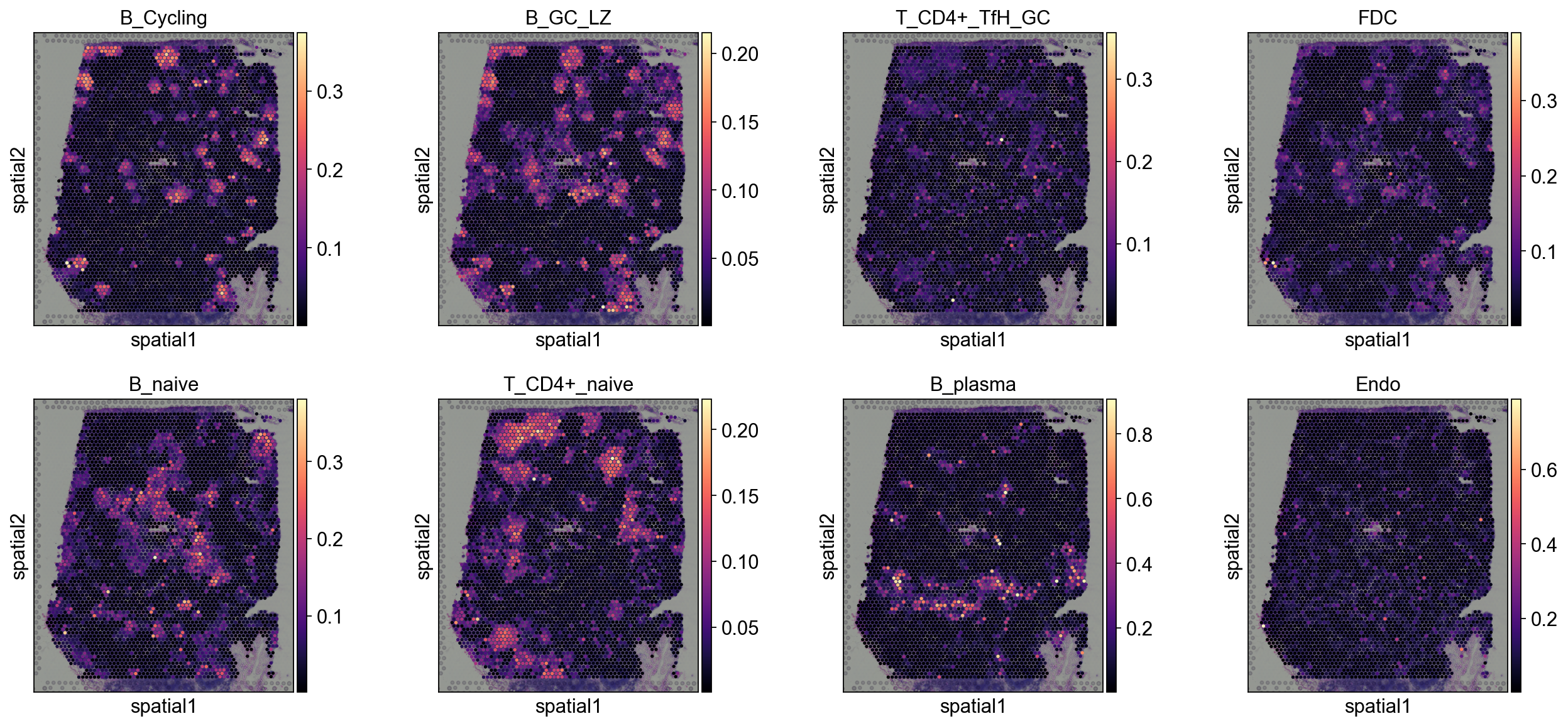
步骤 4: 可视化 (5–15 min)We provide multiple views: single-target spatial heatmaps, multi-target overlays, 和 local pie charts. Start 使用 global inspection, then zoom into biologically relevant regions 对于 higher-resolution assessment.### 4.1 Spatial value dotplot#
annotation_list=['B_Cycling', 'B_GC_LZ', 'T_CD4+_TfH_GC', 'FDC', 'B_naive', 'T_CD4+_naive', 'B_plasma', 'Endo']sc.pl.spatial( decov_obj.adata_cell2location, cmap='magma', # 显示 first 8 细胞类型 颜色=annotation_list, ncols=4, 大小=1.3, img_key='hires', # limit 颜色 缩放 在 99.2% quantile 的 cell abundance #vmin=0, vmax='p99.2')
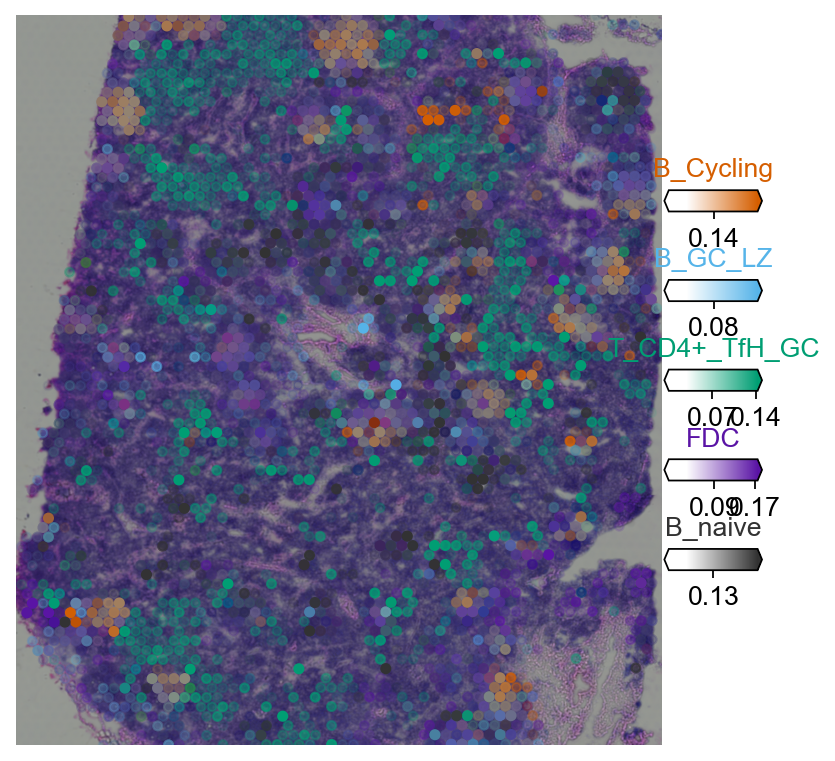
4.2 Multi-target overlay#
import matplotlib as mplclust_labels = annotation_list[:5]clust_col = ['' + str(i) for i in clust_labels] # 在 case column names differ 从 labelswith mpl.rc_context({'图.figsize': (6, 6),'轴.grid': False}): fig = ov.pl.plot_spatial( adata=decov_obj.adata_cell2location, # 标签 到 显示 在 a 绘制 颜色=clust_col, 标签=clust_labels, show_img=True, # 'fast' (white background) 或 'dark_background' style='fast', # limit 颜色 缩放 在 99.2% quantile 的 cell abundance max_color_quantile=0.992, # 大小 的 locations (adjust depending 在 图 大小) circle_diameter=4, reorder_cmap = [#0, 1,2,3,4,6], #['yellow', 'orange', 'blue', 'green', 'purple', 'grey', 'white'], colorbar_position='right', #palette=color_dict )
4.3 Pie plotWe recommend cropping a region 的 interest before plotting 到 avoid overly 密集 pie charts 在 whole slides.#
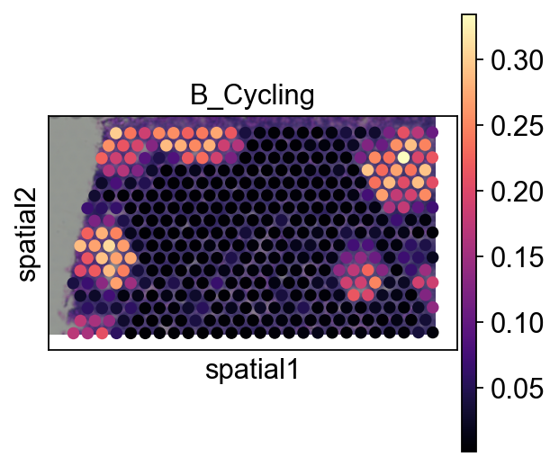
adata_s = ov.space.crop_space_visium( decov_obj.adata_cell2location, crop_loc=(0, 0), crop_area=(500, 1000), library_id=list(decov_obj.adata_cell2location.uns['spatial'].keys())[0] , scale=1)
sc.pl.spatial(adata_s, cmap='magma', # 显示 first 8 细胞类型 颜色=annotation_list[0], ncols=4, 大小=1.3, img_key='hires', # limit 颜色 缩放 在 99.2% quantile 的 cell abundance #vmin=0, vmax='p99.2' )
color_dict=dict(zip(annotation_list, ov.pl.sc_color))
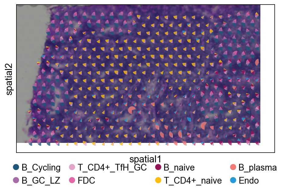
fig, ax = ov.plt.subplots(figsize=(8, 4))sc.pl.spatial( adata_s, basis='spatial', color=None, size=1.3, img_key='hires', ax=ax, show=False)ov.pl.add_pie2spatial( adata_s, img_key='hires', cell_type_columns=annotation_list[:], ax=ax, colors=color_dict, pie_radius=10, remainder='gap', legend_loc=(0.5, -0.25), ncols=4, alpha=0.8)# plt.显示()
<Axes: xlabel='spatial1', ylabel='spatial2'>