Spatial CommunicationSpatial communication is a point of interest for us for the 空间转录组学 Society, and we would like to find the conduction process of spatial communication.Here, we introduce two method integrated in OmicVerse named COMMOT and flowsig.We made three improvements in integrating the COMMOT and flowsig algorithm in OmicVerse:- We reduced the installation conflict of COMMOT and flowsig, user only need to update OmicVerse to the latest version.- We optimized the 可视化 of COMMOT and flowsig and unified the data 预处理 process so that users don’t need to struggle with different data processing flows.- We have fixed some bugs that could occur during function.If you found this tutorial helpful, please cite COMMOT, flowsig and OmicVerse:- Cang, Z., Zhao, Y., Almet, A.A. et al. Screening cell–cell communication in 空间转录组学 via collective optimal transport. Nat Methods 20, 218–228 (2023). https://doi.org/10.1038/s41592-022-01728-4- Almet, A.A., Tsai, YC., Watanabe, M. et al. Inferring pattern-driving intercellular flows from 单细胞 and 空间转录组学. Nat Methods (2024). https://doi.org/10.1038/s41592-024-02380-w

import omicverse as ov# print(f"OmicVerse version: {ov.__version__}")导入 scanpy as sc#print(f"scanpy version: {sc.__version__}")ov.plot_set()

____            _     _    __                  
  / __ \____ ___  (_)___| |  / /__  _____________ 
 / / / / __ `__ \/ / ___/ | / / _ \/ ___/ ___/ _ \ 
/ /_/ / / / / / / / /__ | |/ /  __/ /  (__  )  __/ 
\____/_/ /_/ /_/_/\___/ |___/\___/_/  /____/\___/                                              

Version: 1.6.7, Tutorials: https://omicverse.readthedocs.io/
All dependencies are satisfied.

预处理 dataHere we present our re-analysis of 151676 sample of the dorsolateral prefrontal cortex (DLPFC) dataset. Maynard et al. has manually annotated DLPFC layers and white matter (WM) based on the morphological features and 基因 markers.This tutorial demonstrates how to identify spatial domains on 10x Visium data using STAGATE. The processed data are available at LieberInstitute/spatialLIBD. We downloaded the manual 注释 from the spatialLIBD package and provided at https://drive.google.com/drive/folders/10lhz5VY7YfvHrtV40MwaqLmWz56U9eBP?usp=sharing.

adata = sc.read_visium(path='data', count_file='151676_filtered_feature_bc_matrix.h5')adata.var_names_make_unique()

reading data/151676_filtered_feature_bc_matrix.h5
 (0:00:00)

Note

We introduced the spatial special svg calculation module prost in OmicVerse versions greater than `1.6.0` to replace scanpy's HVGs, if you want to use scanpy's HVGs you can set mode=`scanpy` in `ov.space.svg` or use the following code.

```python#adata=ov.pp.preprocess(adata,mode='shiftlog|pearson',n_HVGs=3000,target_sum=1e4)#adata.raw = adata#adata = adata[:, adata.var.highly_variable_features]```

sc.pp.calculate_qc_metrics(adata, inplace=True)adata = adata[:,adata.var['total_counts']>100]adata=ov.space.svg(adata,mode='prost',n_svgs=3000,target_sum=1e4,platform="visium",)adata

adata.write('data/cluster_svg.h5ad',compression='gzip')

# adata=ov.读取('data/cluster_svg.h5ad',compression='gzip')

Communication Analysis with COMMOT### Spatial communication inferenceWe will use the CellChatDB ligand-receptor database here. Only the secreted signaling LR pairs will be used.Jin, Suoqin, et al. “Inference and analysis of cell-cell communication using CellChat.” Nature communications 12.1 (2021): 1-20.

df_cellchat = ov.external.commot.pp.ligand_receptor_database(species='human',                                                              signaling_type='Secreted Signaling',                                                              database='CellChat')print(df_cellchat.shape)

(1199, 4)

We then 筛选 the LR pairs to keep only the pairs with both ligand and receptor expressed in at least 5% of the spots.

df_cellchat_filtered = ov.external.commot.pp.filter_lr_database(df_cellchat,                                                                 adata,                                                                 min_cell_pct=0.05)print(df_cellchat_filtered.shape)

(19, 4)

Now perform spatial communication inference for these 250 ligand-receptor pairs with a spatial distance limit of 500. CellChat database considers heteromeric units. The signaling results are stored as 点位-by-点位 matrices in the obsp slots. For example, the score for 点位 i signaling to 点位 j through the LR pair can be retrieved from adata.obsp['commot-cellchat-Wnt4-Fzd4_Lrp6'][i,j].

ov.external.commot.tl.spatial_communication(adata,                            database_name='cellchat',                             df_ligrec=df_cellchat_filtered,                             dis_thr=500, heteromeric=True,                             pathway_sum=True)

(Optional) We 读取 the ground truth area of our spatial dataThis step is not mandatory to run, in the tutorial, it’s just to demonstrate the accuracy of our 聚类分析 effect, and in your own tasks, there is often no Ground_truth

Note

You can also use Celltype and other annotated results in adata.obs, here is just a randomly selected type, there is no particular significance, in order to facilitate the 可视化 and study the signal

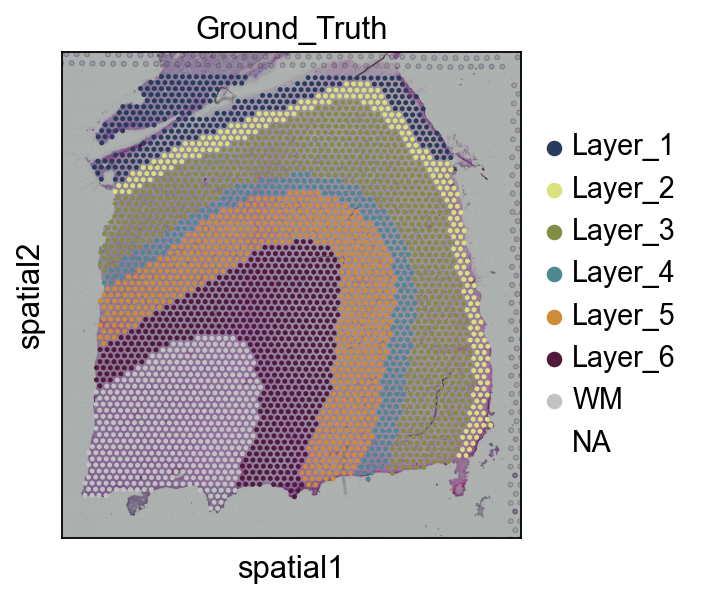
# 读取 the annotationimport Pandas as pdimport osAnn_df = pd.read_csv(os.path.join('data', '151676_truth.txt'), sep='\t', header=None, index_col=0)Ann_df.columns = ['Ground_Truth']adata.obs['Ground_Truth'] = Ann_df.loc[adata.obs_names, 'Ground_Truth']Layer_color=['#283b5c', '#d8e17b', '#838e44', '#4e8991', '#d08c35', '#511a3a',       '#c2c2c2', '#dfc648']sc.pl.spatial(adata, img_key="hires", color=["Ground_Truth"],palette=Layer_color)

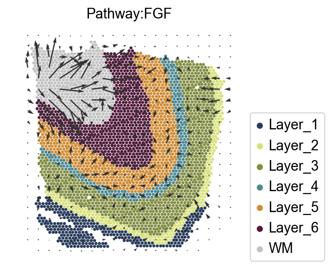
可视化 the communication signal in spatial spaceDetermine the spatial direction of a signaling pathway, for example, the FGF pathway. The interpolated signaling directions for where the signals are sent by the spots and where the signals received by the spots are from are stored in adata.obsm['commot_sender_vf-cellchat-FGF'] and adata.obsm['commot_receiver_vf-cellchat-FGF'], respectively.Taken together, our findings indicate that FGF signaling is crucial for cortical folding in gyrencephalic mammals and is a pivotal upstream regulator of the production of OSVZ progenitors. FGF signaling is the first signaling pathway found to regulate cortical folding.

ct_color_dict=dict(zip(adata.obs['Ground_Truth'].cat.categories,                      adata.uns['Ground_Truth_colors']))

adata.uns['commot-cellchat-info']['df_ligrec'].head()

	ligand	receptor	pathway
0	NRG3	ERBB4	NRG
1	FGF1	FGFR2	FGF
2	FGF1	FGFR3	FGF
3	PDGFA	PDGFRA	PDGF
4	SPP1	ITGAV_ITGB1	SPP1

import matplotlib.pyplot as pltscale=0.000008k=5goal_pathway='FGF'ov.external.commot.tl.communication_direction(adata, database_name='cellchat', pathway_name=goal_pathway, k=k)ov.external.commot.pl.plot_cell_communication(adata, database_name='cellchat',                                               pathway_name='FGF', plot_method='grid',                                               background_legend=True,                                              scale=scale, ndsize=8, grid_density=0.4,                                               summary='sender', background='cluster',                                               clustering='Ground_Truth',                                               cluster_cmap=ct_color_dict,                                              cmap='Alphabet',                                              normalize_v = True, normalize_v_quantile=0.995)plt.title(f'Pathway:{goal_pathway}',fontsize=13)# plt.savefig('figures/TLE/TLE_cellchat_all_FGF.png',dpi=300,bbox_inches='tight')#fig.savefig('pdf/TLE/control_cellchat_all_FGF.pdf',dpi=300,bbox_inches='tight')

Text(0.5, 1.0, 'Pathway:FGF')

adata.write('data/151676_commot.h5ad',compression='gzip')

adata=ov.read('data/151676_commot.h5ad')adata

AnnData object with n_obs × n_vars = 3460 × 5779
    obs: 'in_tissue', 'array_row', 'array_col', 'n_genes_by_counts', 'log1p_n_genes_by_counts', 'total_counts', 'log1p_total_counts', 'pct_counts_in_top_50_genes', 'pct_counts_in_top_100_genes', 'pct_counts_in_top_200_genes', 'pct_counts_in_top_500_genes', 'image_idx_1d', 'Ground_Truth'
    var: 'gene_ids', 'feature_types', 'genome', 'n_cells_by_counts', 'mean_counts', 'log1p_mean_counts', 'pct_dropout_by_counts', 'total_counts', 'log1p_total_counts', 'n_cells', 'SEP', 'SIG', 'PI', 'Moran_I', 'Geary_C', 'p_norm', 'p_rand', 'fdr_norm', 'fdr_rand', 'space_variable_features'
    uns: 'Ground_Truth_colors', 'binary_image', 'commot-cellchat-info', 'del_index', 'gau_fea', 'grid_size', 'locates', 'log1p', 'nor_counts', 'spatial', 'subregions'
    obsm: 'commot-cellchat-sum-receiver', 'commot-cellchat-sum-sender', 'commot_receiver_vf-cellchat-FGF', 'commot_sender_vf-cellchat-FGF', 'spatial'
    layers: 'counts'
    obsp: 'commot-cellchat-ADCYAP1-ADCYAP1R1', 'commot-cellchat-CCK', 'commot-cellchat-CCK-CCKBR', 'commot-cellchat-FGF', 'commot-cellchat-FGF1-FGFR2', 'commot-cellchat-FGF1-FGFR3', 'commot-cellchat-GAS', 'commot-cellchat-GAS6-TYRO3', 'commot-cellchat-GRN', 'commot-cellchat-GRN-SORT1', 'commot-cellchat-NAMPT-INSR', 'commot-cellchat-NRG', 'commot-cellchat-NRG3-ERBB4', 'commot-cellchat-PACAP', 'commot-cellchat-PDGF', 'commot-cellchat-PDGFA-PDGFRA', 'commot-cellchat-PSAP', 'commot-cellchat-PSAP-GPR37', 'commot-cellchat-PSAP-GPR37L1', 'commot-cellchat-PTN', 'commot-cellchat-PTN-NCL', 'commot-cellchat-PTN-PTPRZ1', 'commot-cellchat-PTN-SDC2', 'commot-cellchat-PTN-SDC3', 'commot-cellchat-PTN-SDC4', 'commot-cellchat-SEMATOSTATIN', 'commot-cellchat-SPP1', 'commot-cellchat-SPP1-ITGAV_ITGB1', 'commot-cellchat-SPP1-ITGAV_ITGB5', 'commot-cellchat-SST-SSTR1', 'commot-cellchat-VISFATIN', 'commot-cellchat-total-total'

Communication signal inference with FlowSig### Construct GEMsWe now construct 基因 表达 modules (GEMs) from the unnormalised count data. For ST data, we use NMF.

adata.layers['normalized'] = adata.X.copy()# We construct 10 基因 表达 modules using the raw cell count.ov.external.FlowSig.pp.construct_gems_using_nmf(adata,                                n_gems = 10,                                layer_key = '计数',                                                   )

If you want to study the genes in a GEM, we provide the ov.external.flowsig.ul.get_top_gem_genes function for getting the genes in a specific GEM.

goal_gem='GEM-5'gem_gene=ov.external.flowsig.ul.get_top_gem_genes(adata=adata,                                            gems=[goal_gem],                                         n_genes=100,                                         gene_type='all',                                        method = 'nmf',                                        )gem_gene.head()

	Gene	GEM	Weight
0	PVALB	GEM-5	0.716875
1	CPB1	GEM-5	0.599011
2	GPX3	GEM-5	0.471268
3	SCRT1	GEM-5	0.450501
4	MT-CO2	GEM-5	0.450483

Construct the flow 表达 matricesWe construct augmented flow 表达 matrices for each condition that measure three types of variables:1. Intercellular signal inflow, i.e., how much of a signal did a cell receive. For ST data, signal inflow is constructed by summing the received signals for each significant ligand inferred by COMMOT.2. GEMs, which encapsulate intracellular information processing. We define these as cellwise membership to the GEM.Intercellular signal outflow, i.e., how much of a signal did a cell send. These are simply ligand 基因 表达.3. The kay assumption of FlowSig is that all intercellular information flows are directed from signal inflows to GEMs, from one GEM to another GEM, and from GEMs to signal outflows.For spatial data, we use COMMOT output directly to construct signal inflow 表达 and do not need knowledge about TF databases.

commot_output_key = 'commot-cellchat'# We first construct the potential cellular flows from the COMMOT outputov.external.FlowSig.pp.construct_flows_from_commot(adata,                                commot_output_key,                                gem_expr_key = 'X_gem',                                scale_gem_expr = True,                                flowsig_network_key = 'flowsig_network',                                flowsig_expr_key = 'X_flow')

For spatial data, we retain spatially informative variables, which we determine by calculating the Moran’s I value for signal inflow and signal outflow variables. In case the spatial graph has not been calculated for this data yet, FlowSig will do so, meaning that we need to specify both the coordinate type, grid or generic, and in the case of the former, n_neighs, which in this case, is 8.Flow 表达 variables are defined to be spatially informative if their Moran’s I value is above a specified threshold.

# Then we subset for "spatially flowing" inflows and outflowsov.external.FlowSig.pp.determine_informative_variables(adata,                                      flowsig_expr_key = 'X_flow',                                    flowsig_network_key = 'flowsig_network',                                    spatial = True,                                    moran_threshold = 0.15,                                    coord_type = 'grid',                                    n_neighbours = 8,                                    library_key = None)

Creating graph using `grid` coordinates and `None` transform and `1` libraries.
Adding `adata.obsp['spatial_connectivities']`
       `adata.obsp['spatial_distances']`
       `adata.uns['spatial_neighbors']`
Finish (0:00:00)
Creating graph using `grid` coordinates and `None` transform and `1` libraries.
Adding `adata.obsp['spatial_connectivities']`
       `adata.obsp['spatial_distances']`
       `adata.uns['spatial_neighbors']`
Finish (0:00:00)
Calculating moran's statistic for `None` permutations using `1` core(s)
Adding `adata.uns['moranI']`
Finish (0:00:00)
Calculating moran's statistic for `None` permutations using `1` core(s)
Adding `adata.uns['moranI']`
Finish (0:00:00)

Learn intercellular flowsFor spatial data, where there are far fewer “control vs. perturbed” studies, we use the GSP method, which uses conditional independence testing and a greedy algorithm to learn the CPDAG containing directed arcs and undirected edges.For spatial data, we cannot bootstrap by resampling across individual cells because we would lose the additional layer of correlation contained in the spatial data. Rather, we divide the tissue up into spatial “blocks” and resample within blocks. This is known as block bootstrapping.To 计算 the blocks, we used scikit-learn’s k-means 聚类分析 method to 生成 20 roughly equally sized spatial blocks.

from sklearn.cluster import KMeansimport pandas as pdkmeans = KMeans(n_clusters=10, random_state=0).fit(adata.obsm['spatial'])adata.obs['spatial_kmeans'] = pd.Series(kmeans.labels_, dtype='category').values

We use these blocks to learn the spatial intercellular flows.

# # Now we are ready to learn the networkov.external.FlowSig.tl.learn_intercellular_flows(adata,                        flowsig_key = 'flowsig_network',                        flow_expr_key = 'X_flow',                        use_spatial = True,                        block_key = 'spatial_kmeans',                        n_jobs = 4,                        n_bootstraps = 500)

Partially validate intercellular flow networkFinally, we will remove any “false positive” edges. Noting that the CPDAG contains directed arcs and undirected arcs we do two things.First, we remove directed arcs that are not oriented from signal inflow to GEM, GEM to GEM, or from GEM to signal outflow and for undirected edges, we reorient them so that they obey the previous directionalities.

# This part is key for reducing false positivesov.external.FlowSig.tl.apply_biological_flow(adata,                        flowsig_network_key = 'flowsig_network',                        adjacency_key = 'adjacency',                        validated_key = 'validated')

[[0.    0.    0.    0.03  0.04  0.    0.006 0.    0.002 0.    0.    0.002
  0.002]
 [0.    0.    0.    0.01  0.01  0.004 0.002 0.    0.    0.006 0.    0.
  0.   ]
 [0.    0.    0.    0.002 0.09  0.    0.002 0.002 0.006 0.01  0.    0.002
  0.   ]
 [0.902 1.    0.162 0.    0.094 0.778 0.274 0.598 0.872 0.924 0.356 0.436
  0.304]
 [0.988 1.    0.98  0.158 0.    0.316 0.458 0.428 0.294 0.116 0.528 0.308
  0.294]
 [0.114 0.402 0.    0.368 0.258 0.    0.336 0.24  0.562 0.016 0.048 0.394
  0.128]
 [0.262 0.352 0.028 0.368 0.646 0.78  0.    0.32  0.3   0.04  0.704 0.644
  0.74 ]
 [0.    0.002 0.046 0.578 0.712 0.63  0.22  0.    0.24  0.928 0.624 0.278
  0.728]
 [0.054 0.054 0.352 0.21  0.172 0.492 0.148 0.132 0.    0.618 0.224 0.266
  0.096]
 [0.004 0.15  0.146 0.14  0.024 0.018 0.002 0.132 0.3   0.    0.02  0.042
  0.414]
 [0.034 0.02  0.    0.218 0.564 0.082 0.522 0.55  0.784 0.212 0.    0.562
  0.754]
 [0.174 0.036 0.31  0.302 0.448 0.722 0.514 0.21  0.808 0.248 0.592 0.
  0.764]
 [0.254 0.07  0.    0.198 0.198 0.072 0.296 0.332 0.208 0.6   0.332 0.342
  0.   ]]

Second, we will remove directed arcs whose bootstrapped frequencies are below a specified edge threshold as well as undirected edges whose total bootstrapped frequencies are below the same threshold. Because we did not have perturbation data, we specify a more stringent edge threshold.

edge_threshold = 0.7ov.external.flowsig.tl.filter_low_confidence_edges(adata,                                edge_threshold = edge_threshold,                                flowsig_network_key = 'flowsig_network',                                adjacency_key = 'adjacency_validated',                                filtered_key = 'filtered')

[[0.    0.    0.    0.03  0.04  0.    0.    0.    0.    0.    0.    0.
  0.   ]
 [0.    0.    0.    0.01  0.01  0.    0.    0.    0.    0.    0.    0.
  0.   ]
 [0.    0.    0.    0.    0.09  0.    0.    0.    0.    0.    0.    0.
  0.   ]
 [0.902 1.    0.    0.    0.    0.778 0.    0.598 0.872 0.924 0.    0.436
  0.   ]
 [0.988 1.    0.98  0.    0.    0.    0.458 0.428 0.    0.    0.528 0.308
  0.   ]
 [0.    0.    0.    0.368 0.    0.    0.336 0.24  0.562 0.    0.    0.394
  0.   ]
 [0.    0.    0.    0.    0.646 0.78  0.    0.    0.    0.    0.704 0.644
  0.74 ]
 [0.    0.    0.    0.578 0.712 0.63  0.    0.    0.    0.928 0.624 0.
  0.728]
 [0.    0.    0.    0.21  0.    0.492 0.    0.    0.    0.618 0.224 0.266
  0.   ]
 [0.    0.    0.    0.14  0.    0.    0.    0.132 0.3   0.    0.    0.
  0.414]
 [0.    0.    0.    0.    0.564 0.    0.522 0.55  0.784 0.    0.    0.562
  0.754]
 [0.    0.    0.    0.302 0.448 0.722 0.514 0.    0.808 0.    0.592 0.
  0.764]
 [0.    0.    0.    0.    0.    0.    0.296 0.332 0.    0.6   0.332 0.342
  0.   ]]

adata.write('data/cortex_commot_flowsig.h5ad',compression='gzip')

# adata=ov.读取('data/cortex_commot_flowsig.h5ad')

可视化 the result of flowsigWe can construct the directed NetworkX DiGraph object from adjacency_validated_filtered.

flow_network = ov.external.flowsig.tl.construct_intercellular_flow_network(adata,                                                        flowsig_network_key = 'flowsig_network',                                                        adjacency_key = 'adjacency_validated_filtered')

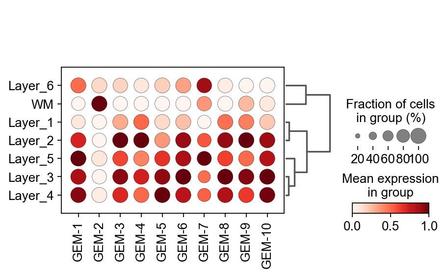
Cell-specific GEMThe first thing we need to be concerned about is which GEM, exactly, is relevant to the cell I want to study. Here, we use dotplot to 可视化 the 表达 of GEM in different cell types.

flowsig_expr_key='X_gem'X_flow = adata.obsm[flowsig_expr_key]adata_subset = sc.AnnData(X=X_flow)adata_subset.obs = adata.obsadata_subset.var.index =[f'GEM-{i}' for i in range(1,len(adata_subset.var)+1)]

import matplotlib.pyplot as pltax=sc.pl.dotplot(adata_subset, adata_subset.var.index, groupby='Ground_Truth',               dendrogram=True,standard_scale='var',cmap='Reds',show=False)color_dict=dict(zip(adata.obs['Ground_Truth'].cat.categories,adata.uns['Ground_Truth_colors']))

WARNING: dendrogram data not found (using key=dendrogram_Ground_Truth). Running `sc.tl.dendrogram` with default parameters. For fine tuning it is recommended to run `sc.tl.dendrogram` independently.
    using data matrix X directly
Storing dendrogram info using `.uns['dendrogram_Ground_Truth']`

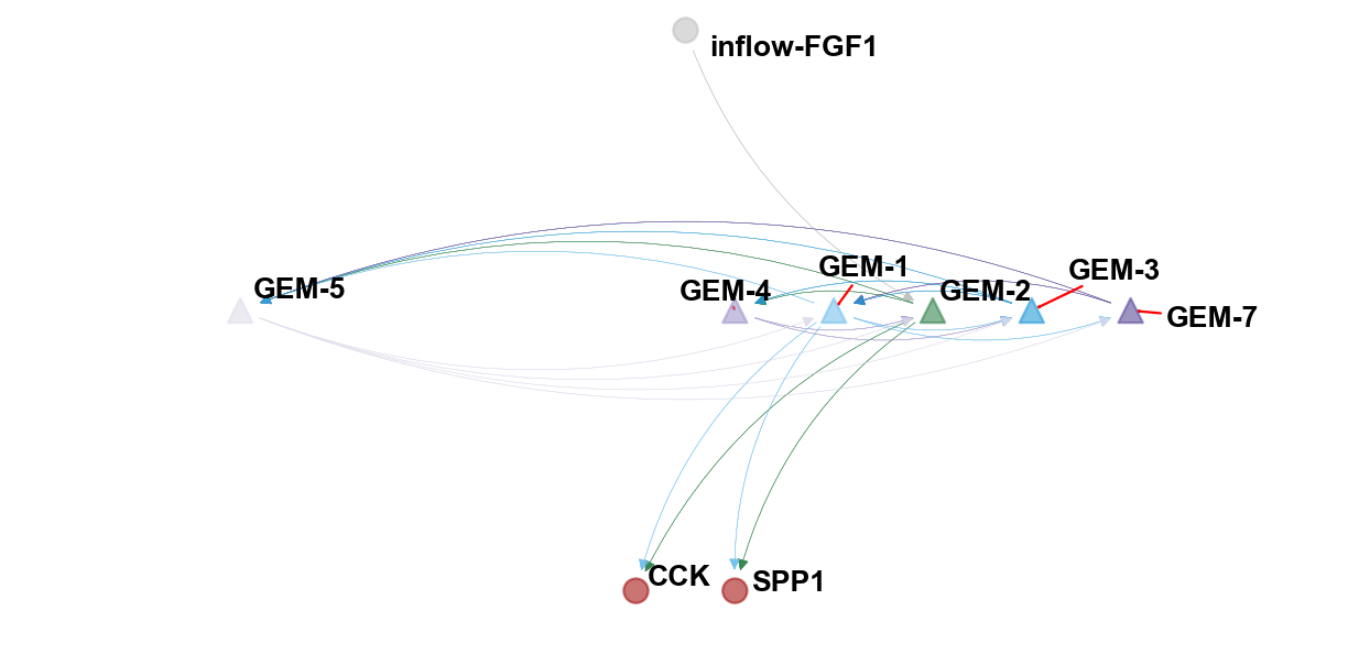
可视化 the FlowSig networkWe fixed the network function provided by the author and provided a better 可视化.

ov.pl.plot_flowsig_network(flow_network=flow_network,                         gem_plot=['GEM-2','GEM-7','GEM-1','GEM-3','GEM-4','GEM-5'],                        figsize=(8,4),                     curve_awarg={'eps':2},                      node_shape={'GEM':'^','Sender':'o','Receptor':'o'},                          ylim=(-0.5,0.5),xlim=(-3,3))

[Text(0.6666666666666666, 0.03418803418803419, 'GEM-1'), Text(-2.0, 0.03418803418803419, 'GEM-5'), Text(1.1111111111111112, 0.03418803418803419, 'GEM-2'), Text(1.5555555555555554, 0.03418803418803419, 'GEM-3'), Text(0.2222222222222222, 0.03418803418803419, 'GEM-4'), Text(2.0, 0.03418803418803419, 'GEM-7'), Text(0.2222222222222222, -0.41025641025641024, 'SPP1'), Text(-0.2222222222222222, -0.41025641025641024, 'CCK'), Text(0.0, 0.4786324786324786, 'inflow-FGF1')]

(<Figure size 640x320 with 1 Axes>, <AxesSubplot: >)