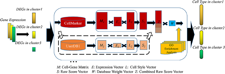
使用 SCSA 进行细胞类型自动注释#
单细胞转录组技术可以在一次实验中分析成千上万个细胞,并识别多种组织和物种中的新型细胞类型、细胞状态及其动态变化。围绕组织单细胞转录组图谱的构建,已经发展出较为标准的实验方案和分析流程。
本教程重点介绍如何解释这类数据,以识别细胞类型、细胞状态以及其他具有生物学意义的模式,从而构建带注释的细胞图谱。
论文: [SCSA: A Cell Type Annotation Tool for Single-Cell RNA-seq Data](https://doi.org/10.3389/fgene.2020.00490
)
Colab 复现: https://colab.research.google.com/drive/1BC6hPS0CyBhNu0BYk8evu57-ua1bAS0T?usp=sharing
注意
SCSA 不适用于稀有细胞类型注释。
import scanpy as sc
print(f'scanpy version:{sc.__version__}')
import omicverse as ov
print(f'omicverse version:{ov.__version__}')
ov.ov_plot_set()
scanpy version:1.11.5
omicverse version:2.1.2rc1
🔬 Starting plot initialization...
🧬 Detecting GPU devices…
✅ Apple Silicon MPS detected
    • [MPS] Apple Silicon GPU - Metal Performance Shaders available

   ____            _     _    __
  / __ \____ ___  (_)___| |  / /__  _____________
 / / / / __ `__ \/ / ___/ | / / _ \/ ___/ ___/ _ \
/ /_/ / / / / / / / /__ | |/ /  __/ /  (__  )  __/
\____/_/ /_/ /_/_/\___/ |___/\___/_/  /____/\___/

🔖 Version: 2.1.2rc1   📚 Tutorials: https://omicverse.readthedocs.io/
✅ plot_set complete.
加载数据#
该数据集由来自一位健康供体的 3k PBMC 组成,可从 10x Genomics 免费获取(可通过这个下载链接或对应的数据页面下载)。在 Unix 系统中,你可以取消下面代码的注释并运行,以下载和解压数据。最后一行会创建一个用于保存处理后数据的目录。
# !mkdir data
# !wget http://cf.10xgenomics.com/samples/cell-exp/1.1.0/pbmc3k/pbmc3k_filtered_gene_bc_matrices.tar.gz -O data/pbmc3k_filtered_gene_bc_matrices.tar.gz
# !cd data; tar -xzf pbmc3k_filtered_gene_bc_matrices.tar.gz
# !mkdir write
将 count matrix 读入 AnnData 对象。AnnData 提供了多个槽位来存储注释信息和不同形式的数据表示,并且自带基于 HDF5 的文件格式:.h5ad。
adata = sc.read_10x_mtx(
    'data/filtered_gene_bc_matrices/hg19/',  # the directory with the `.mtx` file
    var_names='gene_symbols',                # use gene symbols for the variable names (variables-axis index)
    cache=True)                              # write a cache file for faster subsequent reading
数据预处理#
这里我们使用 ov.single.scanpy_lazy 对 scRNA-seq 原始数据进行预处理,流程包括过滤双细胞、按细胞归一化、log1p 转换、提取高变基因以及细胞聚类计算。
如果你希望逐步体验预处理流程,我们也提供了更详细的分步示例,请参考我们的预处理章节。
其中原始 counts 保存在 count layer 中,原始数据本体可通过 adata.raw.to_adata() 访问。
#adata=ov.single.scanpy_lazy(adata)

#quantity control
adata=ov.pp.qc(
    adata,
    tresh={'mito_perc': 0.05, 'nUMIs': 500, 'detected_genes': 250}
)
#normalize and high variable genes (HVGs) calculated
adata=ov.pp.preprocess(adata,mode='shiftlog|pearson',n_HVGs=2000,)

#save the whole genes and filter the non-HVGs
adata.raw = adata
adata = adata[:, adata.var.highly_variable_features]

#scale the adata.X
ov.pp.scale(adata)

#Dimensionality Reduction
ov.pp.pca(adata,layer='scaled',n_pcs=50)

#Neighbourhood graph construction
sc.pp.neighbors(
    adata,
    n_neighbors=15,
    n_pcs=50,
    use_rep='scaled|original|X_pca'
)

#clusters
sc.tl.leiden(adata)

#Dimensionality Reduction for visualization(X_mde=X_umap+GPU)
X_mde = ov.utils.mde(adata.obsm["scaled|original|X_pca"])
if hasattr(X_mde, "detach"):
    X_mde = X_mde.detach().cpu().numpy()
elif hasattr(X_mde, "cpu") and hasattr(X_mde, "numpy"):
    X_mde = X_mde.cpu().numpy()
adata.obsm["X_mde"] = X_mde
adata
🖥️ Using CPU mode for QC...

📊 Step 1: Calculating QC Metrics

   ✓ Gene Family Detection:
   ┌──────────────────────────────┬────────────────────┬────────────────────┐
   │ Gene Family                  │ Genes Found        │ Detection Method   │
   ├──────────────────────────────┼────────────────────┼────────────────────┤
   │ Mitochondrial                │ 13                 │ Auto (MT-)         │
   ├──────────────────────────────┼────────────────────┼────────────────────┤
   │ Ribosomal                    │ 106                │ Auto (RPS/RPL)     │
   ├──────────────────────────────┼────────────────────┼────────────────────┤
   │ Hemoglobin                   │ 13                 │ Auto (regex)       │
   └──────────────────────────────┴────────────────────┴────────────────────┘

   ✓ QC Metrics Summary:
   ┌─────────────────────────┬────────────────────┬─────────────────────────┐
   │ Metric                  │ Mean               │ Range (Min - Max)       │
   ├─────────────────────────┼────────────────────┼─────────────────────────┤
   │ nUMIs                   │ 2367               │ 548 - 15844             │
   ├─────────────────────────┼────────────────────┼─────────────────────────┤
   │ Detected Genes          │ 847                │ 212 - 3422              │
   ├─────────────────────────┼────────────────────┼─────────────────────────┤
   │ Mitochondrial %         │ 2.2%               │ 0.0% - 22.6%            │
   ├─────────────────────────┼────────────────────┼─────────────────────────┤
   │ Ribosomal %             │ 34.9%              │ 1.1% - 59.4%            │
   ├─────────────────────────┼────────────────────┼─────────────────────────┤
   │ Hemoglobin %            │ 0.0%               │ 0.0% - 1.4%             │
   └─────────────────────────┴────────────────────┴─────────────────────────┘

   📈 Original cell count: 2,700

🔧 Step 2: Quality Filtering (SEURAT)
   Thresholds: mito≤0.05, nUMIs≥500, genes≥250
   📊 Seurat Filter Results:
     • nUMIs filter (≥500): 0 cells failed (0.0%)
     • Genes filter (≥250): 3 cells failed (0.1%)
     • Mitochondrial filter (≤0.05): 57 cells failed (2.1%)
   ✓ Filters applied successfully
   ✓ Combined QC filters: 60 cells removed (2.2%)

🎯 Step 3: Final Filtering
   Parameters: min_genes=200, min_cells=3
   Ratios: max_genes_ratio=1, max_cells_ratio=1
   ✓ Final filtering: 0 cells, 19,041 genes removed

🔍 Step 4: Doublet Detection
   ⚠️  Note: 'scrublet' detection is too old and may not work properly
   💡 Consider using 'doublets_method=sccomposite' for better results
   🔍 Running scrublet doublet detection...

🔍 Running Scrublet Doublet Detection:
   Mode: cpu
   Computing doublet prediction using Scrublet algorithm
   🔍 Filtering genes and cells...
🔍 Filtering genes...
   Parameters: min_cells≥3
   ✓ Filtered: 0 genes removed
🔍 Filtering cells...
   Parameters: min_genes≥3
   ✓ Filtered: 0 cells removed
   🔍 Normalizing data and selecting highly variable genes...

🔍 Count Normalization:
   Target sum: median
   Exclude highly expressed: False

✅ Count Normalization Completed Successfully!
   ✓ Processed: 2,640 cells × 13,697 genes
   ✓ Runtime: 0.01s

🔍 Highly Variable Genes Selection:
   Method: seurat
   ⚠️ Gene indices [7846] fell into a single bin: normalized dispersion set to 1
   💡 Consider decreasing `n_bins` to avoid this effect

✅ HVG Selection Completed Successfully!
   ✓ Selected: 1,738 highly variable genes out of 13,697 total (12.7%)
   ✓ Results added to AnnData object:
     • 'highly_variable': Boolean vector (adata.var)
     • 'means': Float vector (adata.var)
     • 'dispersions': Float vector (adata.var)
     • 'dispersions_norm': Float vector (adata.var)
   🔍 Simulating synthetic doublets...
   🔍 Normalizing observed and simulated data...

🔍 Count Normalization:
   Target sum: 1000000.0
   Exclude highly expressed: False

✅ Count Normalization Completed Successfully!
   ✓ Processed: 2,640 cells × 1,738 genes
   ✓ Runtime: 0.00s

🔍 Count Normalization:
   Target sum: 1000000.0
   Exclude highly expressed: False

✅ Count Normalization Completed Successfully!
   ✓ Processed: 5,280 cells × 1,738 genes
   ✓ Runtime: 0.01s
   🔍 Embedding transcriptomes using PCA...
   📊 Scrublet PCA input data type (CPU) - X_obs: ndarray, shape: (2640, 1738), dtype: float64
   📊 Scrublet PCA input data type (CPU) - X_sim: ndarray, shape: (5280, 1738), dtype: float64
   🔍 Calculating doublet scores...
   🔍 Calling doublets with threshold detection...
   📊 Automatic threshold: 0.326
   📈 Detected doublet rate: 1.3%
   🔍 Detectable doublet fraction: 34.0%
   📊 Overall doublet rate comparison:
     • Expected: 5.0%
     • Estimated: 3.9%

✅ Scrublet Analysis Completed Successfully!
   ✓ Results added to AnnData object:
     • 'doublet_score': Doublet scores (adata.obs)
     • 'predicted_doublet': Boolean predictions (adata.obs)
     • 'scrublet': Parameters and metadata (adata.uns)
   ✓ Scrublet completed: 35 doublets removed (1.3%)

╭─ SUMMARY: qc ──────────────────────────────────────────────────────╮
│  Duration: 0.812s                                                  │
│  Shape:    2,700 x 32,738 (Unchanged)                              │
│                                                                    │
│  CHANGES DETECTED                                                  │
│  ────────────────                                                  │
│  ● OBS    │ ✚ cell_complexity (float)                              │
│           │ ✚ detected_genes (int)                                 │
│           │ ✚ hb_perc (float)                                      │
│           │ ✚ mito_perc (float)                                    │
│           │ ✚ nUMIs (float)                                        │
│           │ ✚ passing_mt (bool)                                    │
│           │ ✚ passing_nUMIs (bool)                                 │
│           │ ✚ passing_ngenes (bool)                                │
│           │ ✚ ribo_perc (float)                                    │
│                                                                    │
│  ● VAR    │ ✚ hb (bool)                                            │
│           │ ✚ mt (bool)                                            │
│           │ ✚ ribo (bool)                                          │
│                                                                    │
╰────────────────────────────────────────────────────────────────────╯
🔍 [2026-04-08 19:00:21] Running preprocessing in 'cpu' mode...
Begin robust gene identification
    After filtration, 13697/13697 genes are kept.
    Among 13697 genes, 13696 genes are robust.
✅ Robust gene identification completed successfully.
Begin size normalization: shiftlog and HVGs selection pearson

🔍 Count Normalization:
   Target sum: 500000.0
   Exclude highly expressed: True
   Max fraction threshold: 0.2
   ⚠️ Excluding 0 highly-expressed genes from normalization computation
   Excluded genes: []

✅ Count Normalization Completed Successfully!
   ✓ Processed: 2,605 cells × 13,696 genes
   ✓ Runtime: 0.04s

🔍 Highly Variable Genes Selection (Experimental):
   Method: pearson_residuals
   Target genes: 2,000
   Theta (overdispersion): 100

✅ Experimental HVG Selection Completed Successfully!
   ✓ Selected: 2,000 highly variable genes out of 13,696 total (14.6%)
   ✓ Results added to AnnData object:
     • 'highly_variable': Boolean vector (adata.var)
     • 'highly_variable_rank': Float vector (adata.var)
     • 'highly_variable_nbatches': Int vector (adata.var)
     • 'highly_variable_intersection': Boolean vector (adata.var)
     • 'means': Float vector (adata.var)
     • 'variances': Float vector (adata.var)
     • 'residual_variances': Float vector (adata.var)
    Time to analyze data in cpu: 0.12 seconds.
✅ Preprocessing completed successfully.
    Added:
        'highly_variable_features', boolean vector (adata.var)
        'means', float vector (adata.var)
        'variances', float vector (adata.var)
        'residual_variances', float vector (adata.var)
        'counts', raw counts layer (adata.layers)
    End of size normalization: shiftlog and HVGs selection pearson

╭─ SUMMARY: preprocess ──────────────────────────────────────────────╮
│  Duration: 0.1281s                                                 │
│  Shape:    2,605 x 13,697 -> 2,605 x 13,696                        │
│                                                                    │
│  CHANGES DETECTED                                                  │
│  ────────────────                                                  │
│  ● VAR    │ ✚ highly_variable (bool)                               │
│           │ ✚ highly_variable_features (bool)                      │
│           │ ✚ highly_variable_rank (float)                         │
│           │ ✚ means (float)                                        │
│           │ ✚ n_cells (int)                                        │
│           │ ✚ percent_cells (float)                                │
│           │ ✚ residual_variances (float)                           │
│           │ ✚ robust (bool)                                        │
│           │ ✚ variances (float)                                    │
│                                                                    │
│  ● UNS    │ ✚ history_log                                          │
│           │ ✚ hvg                                                  │
│           │ ✚ log1p                                                │
│                                                                    │
│  ● LAYERS │ ✚ counts (sparse matrix, 2605x13696)                   │
│                                                                    │
╰────────────────────────────────────────────────────────────────────╯
    Converting scaled data to csr_matrix format...

╭─ SUMMARY: scale ───────────────────────────────────────────────────╮
│  Duration: 0.0872s                                                 │
│  Shape:    2,605 x 2,000 (Unchanged)                               │
│                                                                    │
│  CHANGES DETECTED                                                  │
│  ────────────────                                                  │
│  ● LAYERS │ ✚ scaled (sparse matrix, 2605x2000)                    │
│                                                                    │
╰────────────────────────────────────────────────────────────────────╯
computing PCA🔍
    with n_comps=50
   🖥️ Using sklearn PCA for CPU computation
   🖥️ sklearn PCA backend: CPU computation
   📊 PCA input data type: SparseCSRMatrixView, shape: (2605, 2000), dtype: float64
   📊 Sparse matrix density: 100.00%
   🔧 PCA solver used: covariance_eigh
    finished✅ (16.44s)

╭─ SUMMARY: pca ─────────────────────────────────────────────────────╮
│  Duration: 16.4474s                                                │
│  Shape:    2,605 x 2,000 (Unchanged)                               │
│                                                                    │
│  CHANGES DETECTED                                                  │
│  ────────────────                                                  │
│  ● UNS    │ ✚ pca                                                  │
│           │ └─ params: {'zero_center': True, 'use_highly_variable': Tr...│
│           │ ✚ scaled|original|cum_sum_eigenvalues                  │
│           │ ✚ scaled|original|pca_var_ratios                       │
│                                                                    │
│  ● OBSM   │ ✚ X_pca (array, 2605x50)                               │
│           │ ✚ scaled|original|X_pca (array, 2605x50)               │
│                                                                    │
╰────────────────────────────────────────────────────────────────────╯
AnnData object with n_obs × n_vars = 2605 × 2000
    obs: 'nUMIs', 'mito_perc', 'ribo_perc', 'hb_perc', 'detected_genes', 'cell_complexity', 'passing_mt', 'passing_nUMIs', 'passing_ngenes', 'doublet_score', 'predicted_doublet', 'leiden'
    var: 'gene_ids', 'mt', 'ribo', 'hb', 'n_cells', 'percent_cells', 'robust', 'highly_variable_features', 'means', 'variances', 'residual_variances', 'highly_variable_rank', 'highly_variable'
    uns: 'scrublet', 'status', 'status_args', 'REFERENCE_MANU', 'history_log', 'log1p', 'hvg', 'pca', 'scaled|original|pca_var_ratios', 'scaled|original|cum_sum_eigenvalues', 'neighbors', 'leiden'
    obsm: 'X_pca', 'scaled|original|X_pca', 'X_mde'
    varm: 'PCs', 'scaled|original|pca_loadings'
    layers: 'counts', 'scaled'
    obsp: 'distances', 'connectivities'
自动细胞注释#
我们基于 adata 创建一个 pySCSA 对象,并设置若干参数以获得正确的注释结果。
在常规注释任务中,通常将 celltype 设为 'normal',并将 target 设为 'cellmarker' 或 'panglaodb' 来进行细胞类型注释。
而在肿瘤注释任务中,则需要将 celltype 设为 'cancer',并将 target 设为 'cancersea'。
说明
使用 SCSA 进行注释前需要先下载数据库。通常可以自动下载,但在某些网络环境下可能会遇到下载失败的问题。
2023 版本(基于 pandas<=1.5.3):数据库可从 figshare、Google Drive 和 百度云 下载。
2024 版本(基于 pandas>2):数据库可从 Google Drive 和 百度云 下载。
并且你需要将参数 model_path 设置为对应数据库文件路径。
数据库构建代码可参考 scsa_database_create.ipynb。感谢 @fredsamhaak 与 @H1207953831 在 issue #232 和 #176 中的讨论与帮助。
scsa=ov.single.pySCSA(
    adata=adata,
    foldchange=1.5,
    pvalue=0.01,
    celltype='normal',
    target='cellmarker',
    tissue='All',
    model_path='temp/pySCSA_2024_v1_plus.db'
)
在前面的聚类步骤中,我们使用的是 leiden 算法,因此这里将聚类类型指定为 leiden。如果你使用的是 louvain,请相应修改该参数。另外,这里会对所有 cluster 进行注释;如果你只想注释部分 cluster,可按 '[1]'、'[1,2,3]'、'[...]' 这样的格式输入。
rank_rep 对应 sc.tl.rank_genes_groups(adata, clustertype, method='wilcoxon') 的计算过程;如果你的 adata.uns 中已经包含 rank_genes_groups 结果,则可将 rank_rep 设为 False。
anno=scsa.cell_anno(
    clustertype='leiden',
    cluster='all',
    rank_rep=True
)
ranking genes
finished (0:00:00)
...Auto annotate cell
🔍 Version V2.2 [2024/12/18]
📊 DB load: GO_items:47347, Human_GO:3, Mouse_GO:3,
CellMarkers:82887, CancerSEA:1574, PanglaoDB:24223
Ensembl_HGNC:61541, Ensembl_Mouse:55414
<omicverse.single._SCSA.Annotator object at 0x13051f690>
🔍 Version V2.2 [2024/12/18]
📊 DB load: GO_items:47347, Human_GO:3, Mouse_GO:3,
CellMarkers:82887, CancerSEA:1574, PanglaoDB:24223
Ensembl_HGNC:61541, Ensembl_Mouse:55414
📦 Load markers: 70276
============================================================
🔬 Analyzing 9 clusters...
============================================================
[1/9] Cluster 0 │ 75 genes │ 1351 other genes
[2/9] Cluster 1 │ 154 genes │ 1292 other genes
[3/9] Cluster 2 │ 581 genes │ 1250 other genes
[4/9] Cluster 3 │ 128 genes │ 1307 other genes
[5/9] Cluster 4 │ 81 genes │ 1370 other genes
[6/9] Cluster 5 │ 908 genes │ 989 other genes
[7/9] Cluster 6 │ 256 genes │ 1265 other genes
[8/9] Cluster 7 │ 52 genes │ 1384 other genes
[9/9] Cluster 8 │ 5 genes │ 1384 other genes
============================================================
✅ Cluster analysis completed! (9/9 processed)
============================================================
================================================================================
📋 Cell Type Annotation Results
================================================================================
Cluster Type Cell Type Score Times
--------------------------------------------------------------------------------
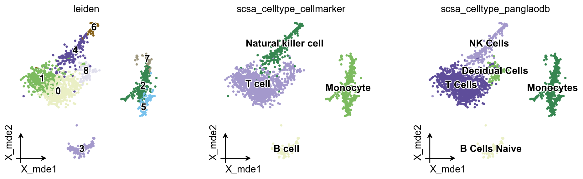
0 ⚠️ ? T cell|Naive CD8+ T cell 8.781928906119388|5.3060528449921955 1.66
1 ✅ Good T cell 13.575245113590226 2.07
2 ⚠️ ? Monocyte|Macrophage 14.798208690107241|8.829828211698532 1.68
3 ✅ Good B cell 13.794561862211818 4.00
4 ⚠️ ? Natural killer cell|T cell 9.334956049479073|7.343244933648183 1.27
5 ⚠️ ? Monocyte|Macrophage 13.918759306986406|10.037946625130374 1.39
6 ✅ Good Natural killer cell 15.30826245310867 3.40
7 ✅ Good Monocyte 10.787406042786724 2.18
8 ⚠️ ? T cell|CD8+ T cell 5.431184801334877|4.133502801071792 1.31
================================================================================
我们可以只查看注释质量较好的结果。
scsa.cell_auto_anno(adata,key='scsa_celltype_cellmarker')
...cell type added to scsa_celltype_cellmarker on obs of anndata
我们也可以使用 panglaodb 作为 target 来进行细胞类型注释。
scsa=ov.single.pySCSA(
    adata=adata,
    foldchange=1.5,
    pvalue=0.01,
    celltype='normal',
    target='panglaodb',
    tissue='All',
    model_path='temp/pySCSA_2024_v1_plus.db'
)
res=scsa.cell_anno(
    clustertype='leiden',
    cluster='all',
    rank_rep=True
)
ranking genes
    finished (0:00:00)
...Auto annotate cell
🔍 Version V2.2 [2024/12/18]
📊 DB load: GO_items:47347, Human_GO:3, Mouse_GO:3,
           CellMarkers:82887, CancerSEA:1574, PanglaoDB:24223
           Ensembl_HGNC:61541, Ensembl_Mouse:55414
<omicverse.single._SCSA.Annotator object at 0x14c448050>
🔍 Version V2.2 [2024/12/18]
📊 DB load: GO_items:47347, Human_GO:3, Mouse_GO:3,
           CellMarkers:82887, CancerSEA:1574, PanglaoDB:24223
           Ensembl_HGNC:61541, Ensembl_Mouse:55414
📦 Load markers: 70276

============================================================
🔬 Analyzing 9 clusters...
============================================================

[1/9]      Cluster 0    │ 75   genes │ 632  other genes
[2/9]      Cluster 1    │ 154  genes │ 602  other genes
[3/9]      Cluster 2    │ 581  genes │ 572  other genes
[4/9]      Cluster 3    │ 128  genes │ 592  other genes
[5/9]      Cluster 4    │ 81   genes │ 635  other genes
[6/9]      Cluster 5    │ 908  genes │ 538  other genes
[7/9]      Cluster 6    │ 256  genes │ 586  other genes
[8/9]      Cluster 7    │ 52   genes │ 645  other genes
[9/9]      Cluster 8    │ 5    genes │ 645  other genes

============================================================
✅ Cluster analysis completed! (9/9 processed)
============================================================


================================================================================
📋 Cell Type Annotation Results
================================================================================

Cluster    Type     Cell Type                           Score           Times
--------------------------------------------------------------------------------
0          ⚠️ ?      T Cells|T Memory Cells              3.7202138087000143|3.3571403840625624 1.11
1          ⚠️ ?      T Cells|T Memory Cells              3.5389401028805043|3.109624332162554 1.14
2          ⚠️ ?      Monocytes|Alveolar Macrophages      3.6648210820925704|2.9377520436871687 1.25
3          ⚠️ ?      B Cells Naive|B Cells Memory        4.335481613464625|3.9591672199193098 1.10
4          ⚠️ ?      NK Cells|T Cells                    2.9343417206491886|2.5083417903196352 1.17
5          ⚠️ ?      Monocytes|Macrophages               3.762558876283017|2.8175042671102175 1.34
6          ⚠️ ?      NK Cells|Gamma Delta T Cells        4.052418431477111|2.8660094064808934 1.41
7          ⚠️ ?      Monocytes|Alveolar Macrophages      2.597715597444312|2.1244779821849584 1.22
8          ⚠️ ?      Decidual Cells|NK Cells             1.629486719474794|1.629486719474794 1.00
================================================================================
我们同样可以只查看注释质量较好的结果。
scsa.cell_anno_print()
Cluster:0	Cell_type:T Cells|T Memory Cells	Z-score:3.72|3.357
Cluster:1	Cell_type:T Cells|T Memory Cells	Z-score:3.539|3.11
Cluster:2	Cell_type:Monocytes|Alveolar Macrophages	Z-score:3.665|2.938
Cluster:3	Cell_type:B Cells Naive|B Cells Memory	Z-score:4.335|3.959
Cluster:4	Cell_type:NK Cells|T Cells	Z-score:2.934|2.508
Cluster:5	Cell_type:Monocytes|Macrophages	Z-score:3.763|2.818
Cluster:6	Cell_type:NK Cells|Gamma Delta T Cells	Z-score:4.052|2.866
Cluster:7	Cell_type:Monocytes|Alveolar Macrophages	Z-score:2.598|2.124
Cluster:8	Cell_type:Decidual Cells|NK Cells	Z-score:1.629|1.629
scsa.cell_auto_anno(adata,key='scsa_celltype_panglaodb')
...cell type added to scsa_celltype_panglaodb on obs of anndata
这里介绍降维可视化函数 ov.utils.embedding。它与 scanpy.pl.embedding 类似,不同之处在于当设置 frameon='small' 时,坐标轴会缩放到左下角,颜色条会缩放到右下角。
adata: anndata 对象
basis: 存储在
adata.obsm中、用于展示的嵌入坐标color: 需要可视化的 obs/var 信息
legend_loc: 图例位置;若设为
None,会显示在右侧frameon: 可以设置为
small、False或Nonelegend_fontoutline: 图例文字描边宽度
palette: 用于指定不同类别的颜色。除了 omicverse 的默认调色板外,也可以像下面这样直接传入颜色字典,以获得更稳定的显示效果。
ov.utils.embedding(
    adata,
    basis='X_mde',
    color=['leiden','scsa_celltype_cellmarker','scsa_celltype_panglaodb'],
    legend_loc='on data',
    frameon='small',
    legend_fontoutline=2,
    palette=ov.utils.palette()[9:],
)
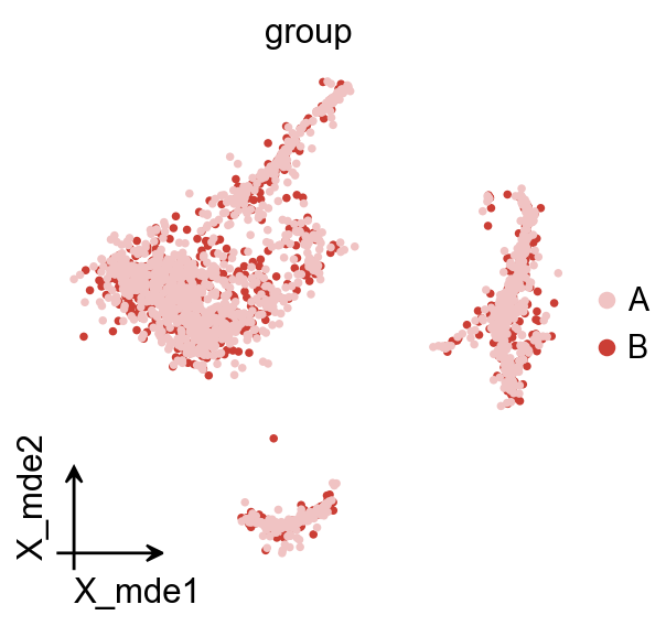
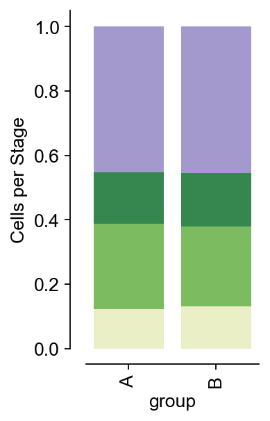
如果你想绘制细胞类型比例的堆叠柱状图,首先需要使用 ov.utils.embedding 对待比较的分组进行着色,然后再使用 ov.utils.plot_cellproportion 指定要展示的分组,即可查看不同组中的细胞比例。
# 随机将前 1000 个细胞标记为 B 组,其余细胞标记为 A 组
adata.obs['group']='A'
adata.obs.loc[adata.obs.index[:1000],'group']='B'
# 着色展示
ov.utils.embedding(
    adata,
    basis='X_mde',
    color=['group'],
    frameon='small',
    legend_fontoutline=2,
    palette={'A': '#F0C3C3', 'B': '#CB3E35'},
)
ov.utils.plot_cellproportion(
    adata=adata,
    celltype_clusters='scsa_celltype_cellmarker',
    visual_clusters='group',
    visual_name='group',
    figsize=(2,4)
)
(<Figure size 160x320 with 1 Axes>,
 <Axes: xlabel='group', ylabel='Cells per Stage'>)
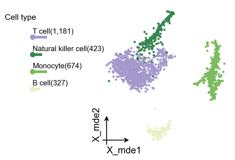
当然,我们还提供了另一种缩略式的嵌入图可视化函数 ov.utils.plot_embedding_celltype。
ov.utils.plot_embedding_celltype(
    adata,
    figsize=None,
    basis='X_mde',
    celltype_key='scsa_celltype_cellmarker',
    title='Cell type',
    celltype_range=(2,6),
    embedding_range=(4,10)
)
(<Figure size 480x320 with 2 Axes>,
 [<Axes: xlabel='X_mde1', ylabel='X_mde2'>, <Axes: >])
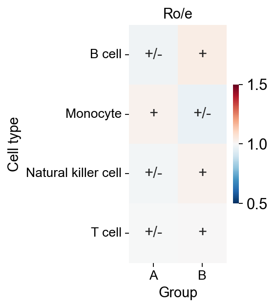
我们计算了不同组织中每个簇的观测细胞数与期望细胞数之比(Ro/e),以量化每个簇的组织偏好性(Guo et al., 2018; Zhang et al., 2018)。细胞簇与组织组合对应的期望细胞数由卡方检验得到。当某个簇在特定组织中的 Ro/e > 1 时,可以认为该簇在该组织中富集。
Ro/e 相关函数由 Haihao Zhang 编写。
roe=ov.utils.roe(
    adata,
    sample_key='group',
    cell_type_key='scsa_celltype_cellmarker'
)
chi2: 0.8694929746430213, dof: 3, pvalue: 0.8327829060823263
P-value is greater than 0.05, there is no statistical significance
import seaborn as sns
import matplotlib.pyplot as plt
fig, ax = plt.subplots(figsize=(2,4))

transformed_roe = roe.copy()
transformed_roe = transformed_roe.applymap(
    lambda x: '+++' if x >= 2 else ('++' if x >= 1.5 else ('+' if x >= 1 else '+/-')))

sns.heatmap(
    roe,
    annot=transformed_roe,
    cmap='RdBu_r',
    fmt='',
    cbar=True,
    ax=ax,
    vmin=0.5,
    vmax=1.5,
    cbar_kws={'shrink':0.5}
)
plt.xticks(fontsize=12)
plt.yticks(fontsize=12)

plt.xlabel('Group',fontsize=13)
plt.ylabel('Cell type',fontsize=13)
plt.title('Ro/e',fontsize=13)
Text(0.5, 1.0, 'Ro/e')
手动细胞注释#
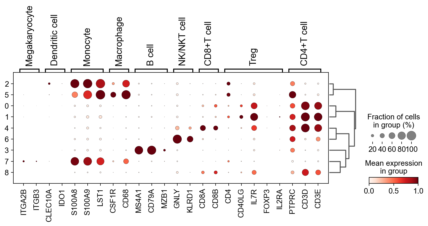
为了比较自动注释结果的准确性,这里我们将使用 marker genes 对各个簇进行手动注释,并将手动注释结果与 pySCSA 的结果进行对比。
首先需要准备一个 marker 基因字典。
res_marker_dict={
    'Megakaryocyte':['ITGA2B','ITGB3'],
    'Dendritic cell':['CLEC10A','IDO1'],
    'Monocyte' :['S100A8','S100A9','LST1',],
    'Macrophage':['CSF1R','CD68'],
    'B cell':['MS4A1','CD79A','MZB1',],
    'NK/NKT cell':['GNLY','KLRD1'],
    'CD8+T cell':['CD8A','CD8B'],
    'Treg':['CD4','CD40LG','IL7R','FOXP3','IL2RA'],
    'CD4+T cell':['PTPRC','CD3D','CD3E'],
}
接着,我们计算每个簇中 marker genes 的表达水平及其表达比例。
sc.tl.dendrogram(adata,'leiden')
sc.pl.dotplot(
    adata,
    res_marker_dict,
    'leiden',
    dendrogram=True,
    standard_scale='var'
)
using 'X_pca' with n_pcs = 50
Storing dendrogram info using `.uns['dendrogram_leiden']`
WARNING: Groups are not reordered because the `groupby` categories and the `var_group_labels` are different.
categories: 0, 1, 2, etc.
var_group_labels: Megakaryocyte, Dendritic cell, Monocyte, etc.
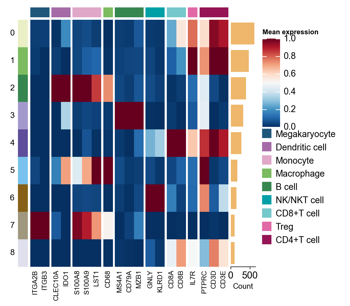
我们也可以使用基于 Marsilea 的新分组热图来展示同一批 marker genes。
marker_genes_heatmap = {k: v for k, v in res_marker_dict.items() if len(v) > 0}
h = ov.pl.group_heatmap(
    adata,
    var_names=marker_genes_heatmap,
    groupby='leiden',
    figsize=(4, 5),
    standard_scale='var',
    cmap='RdBu_r',
    border=False,
    show=False
)
基于 dotplot 的结果,我们使用 ov.single.scanpy_cellanno_from_dict 为每个簇指定名称。
# 创建簇到注释标签的映射字典
cluster2annotation = {
    '0': 'T cell',
    '1': 'T cell',
    '2': 'Monocyte', # Germ-cell(Oid)
    '3': 'B cell',   # Germ-cell(Oid)
    '4': 'T cell',
    '5': 'Macrophage',
    '6': 'NKT cells',
    '7': 'Monocyte',
    '8': 'T cell',
    '9': 'Dendritic cell',
    '10':'Megakaryocyte',
}
ov.single.scanpy_cellanno_from_dict(
    adata,anno_dict=cluster2annotation,
    clustertype='leiden'
)
...cell type added to major_celltype on obs of anndata
比较 pySCSA 与手动注释#
可以看到,自动注释结果与手动注释结果几乎一致,唯一的差异主要出现在 monocyte 与 macrophage 的区分上。不过在前面的自动注释结果中,pySCSA 也给出了 monocyte|macrophage 这样的候选结果,因此可以认为 pySCSA 在 pbmc3k 数据上的表现仍然较好。
ov.utils.embedding(
    adata,
    basis='X_mde',
    color=['leiden','major_celltype','scsa_celltype_cellmarker'],
    legend_loc='on data',
    frameon='small',
    legend_fontoutline=2,
    palette=ov.utils.palette()[9:],
)
我们也可以使用 ov.pl.cell_cor_heatmap 来比较手动注释结果与 pySCSA 自动注释结果之间的表达相似性。
cell_cor_h = ov.pl.cell_cor_heatmap(
    adata,
    group_by='major_celltype',
    ref_adata=adata,
    ref_group_by='scsa_celltype_cellmarker',
    method='pearson',
    standard_scale='var',
    cmap='RdBu_r',
    figsize=(2, 2.5),
    row_cluster=True,
    col_cluster=True,
    show_values=True,
    value_cutoff=0.3,
    border=False,
    show=False,
)
我们可以使用 get_celltype_marker 获取每种细胞类型对应的 marker genes。
marker_dict=ov.single.get_celltype_marker(adata,clustertype='scsa_celltype_cellmarker')
marker_dict.keys()
...get cell type marker
ranking genes
    finished (0:00:00)
dict_keys(['B cell', 'Monocyte', 'Natural killer cell', 'T cell'])
marker_dict['B cell']
['CD37',
 'HLA-DPB1',
 'HLA-DQA1',
 'CD74',
 'MS4A1',
 'HLA-DRB1',
 'HLA-DRA',
 'CD79B',
 'HLA-DQB1',
 'CD79A']
数据库中的组织名称#
如果需要对特定组织中的细胞类型进行注释,可以使用 get_model_tissue 查询数据库中可用的组织名称。
scsa.get_model_tissue()
🔍 Version V2.2 [2024/12/18]
📊 DB load: GO_items:47347, Human_GO:3, Mouse_GO:3,
           CellMarkers:82887, CancerSEA:1574, PanglaoDB:24223
           Ensembl_HGNC:61541, Ensembl_Mouse:55414
########################################################################################################################
------------------------------------------------------------------------------------------------------------------------
Species:Human      Num:298
------------------------------------------------------------------------------------------------------------------------
  1: Abdomen                              2: Abdominal adipose tissue             3: Abdominal fat pad
  4: Acinus                               5: Adipose tissue                       6: Adrenal gland
  7: Adventitia                           8: Airway                               9: Airway epithelium
 10: Allocortex                          11: Alveolus                            12: Amniotic fluid
 13: Amniotic membrane                   14: Ampullary                           15: Anogenital tract
 16: Antecubital vein                    17: Anterior cruciate ligament          18: Anterior presomitic mesoderm
 19: Aorta                               20: Aortic valve                        21: Artery
 22: Arthrosis                           23: Articular Cartilage                 24: Ascites
 25: Ascitic fluid                       26: Atrium                              27: Basal airway
 28: Basilar membrane                    29: Beige Fat                           30: Bile duct
 31: Biliary tract                       32: Bladder                             33: Blood
 34: Blood vessel                        35: Bone                                36: Bone marrow
 37: Brain                               38: Breast                              39: Bronchial vessel
 40: Bronchiole                          41: Bronchoalveolar lavage              42: Bronchoalveolar system
 43: Bronchus                            44: Brown adipose tissue                45: Calvaria
 46: Capillary                           47: Cardiac atrium                      48: Cardiovascular system
 49: Carotid artery                      50: Carotid plaque                      51: Cartilage
 52: Caudal cortex                       53: Caudal forebrain                    54: Caudal ganglionic eminence
 55: Cavernosum                          56: Central amygdala                    57: Central nervous system
 58: Cerebellum                          59: Cerebral organoid                   60: Cerebrospinal fluid
 61: Cervix                              62: Choriocapillaris                    63: Chorionic villi
 64: Chorionic villus                    65: Choroid                             66: Choroid plexus
 67: Colon                               68: Colon epithelium                    69: Colorectum
 70: Cornea                              71: Corneal endothelium                 72: Corneal epithelium
 73: Coronary artery                     74: Corpus callosum                     75: Corpus luteum
 76: Cortex                              77: Cortical layer                      78: Cortical thymus
 79: Decidua                             80: Deciduous tooth                     81: Dental pulp
 82: Dermis                              83: Diencephalon                        84: Distal airway
 85: Dorsal forebrain                    86: Dorsal root ganglion                87: Dorsolateral prefrontal cortex
 88: Ductal tissue                       89: Duodenum                            90: Ectocervix
 91: Ectoderm                            92: Embryo                              93: Embryoid body
 94: Embryonic Kidney                    95: Embryonic brain                     96: Embryonic heart
 97: Embryonic prefrontal cortex         98: Embryonic stem cell                 99: Endocardium
100: Endocrine                          101: Endoderm                           102: Endometrium
103: Endometrium stroma                 104: Entorhinal cortex                  105: Epidermis
106: Epithelium                         107: Esophageal                         108: Esophagus
109: Eye                                110: Fat pad                            111: Fetal brain
112: Fetal gonad                        113: Fetal heart                        114: Fetal ileums
115: Fetal kidney                       116: Fetal liver                        117: Fetal lung
118: Fetal thymus                       119: Fetal umbilical cord               120: Fetus
121: Foreskin                           122: Frontal cortex                     123: Fundic gland
124: Gall bladder                       125: Gastric corpus                     126: Gastric epithelium
127: Gastric gland                      128: Gastrointestinal tract             129: Germ
130: Germinal center                    131: Gingiva                            132: Gonad
133: Gut                                134: Hair follicle                      135: Head
136: Head and neck                      137: Heart                              138: Heart muscle
139: Hippocampus                        140: Ileum                              141: Iliac crest
142: Inferior colliculus                143: Intervertebral disc                144: Intestinal crypt
145: Intestine                          146: Intrahepatic cholangio             147: Jejunum
148: Kidney                             149: Lacrimal gland                     150: Large Intestine
151: Large intestine                    152: Larynx                             153: Lateral ganglionic eminence
154: Left lobe                          155: Ligament                           156: Limb bud
157: Limbal epithelium                  158: Liver                              159: Lumbar vertebra
160: Lung                               161: Lymph                              162: Lymph node
163: Lymphatic vessel                   164: Lymphoid tissue                    165: Malignant pleural effusion
166: Mammary epithelium                 167: Mammary gland                      168: Medial ganglionic eminence
169: Medullary thymus                   170: Meniscus                           171: Mesenchyme
172: Mesoblast                          173: Mesoderm                           174: Microvascular endothelium
175: Microvessel                        176: Midbrain                           177: Middle temporal gyrus
178: Milk                               179: Molar                              180: Muscle
181: Myenteric plexus                   182: Myocardium                         183: Myometrium
184: Nasal concha                       185: Nasal epithelium                   186: Nasal mucosa
187: Nasal polyp                        188: Nasopharyngeal mucosa              189: Nasopharynx
190: Neck                               191: Neocortex                          192: Nerve
193: Nose                               194: Nucleus pulposus                   195: Olfactory neuroepithelium
196: Omentum                            197: Optic nerve                        198: Oral cavity
199: Oral mucosa                        200: Osteoarthritic cartilage           201: Ovarian cortex
202: Ovarian follicle                   203: Ovary                              204: Oviduct
205: Palatine tonsil                    206: Pancreas                           207: Pancreatic acinar tissue
208: Pancreatic duct                    209: Pancreatic islet                   210: Periodontal ligament
211: Periodontium                       212: Periosteum                         213: Peripheral blood
214: Peritoneal fluid                   215: Peritoneum                         216: Pituitary
217: Pituitary gland                    218: Placenta                           219: Plasma
220: Pleura                             221: Pluripotent stem cell              222: Polyp
223: Posterior fossa                    224: Posterior presomitic mesoderm      225: Prefrontal cortex
226: Premolar                           227: Presomitic mesoderm                228: Primitive streak
229: Prostate                           230: Pulmonary arteriy                  231: Pyloric gland
232: Rectum                             233: Renal glomerulus                   234: Respiratory tract
235: Retina                             236: Retinal organoid                   237: Retinal pigment epithelium
238: Right ventricle                    239: Saliva                             240: Salivary gland
241: Scalp                              242: Sclerocorneal tissue               243: Seminal plasma
244: Septum transversum                 245: Serum                              246: Sinonasal mucosa
247: Sinus tissue                       248: Skeletal muscle                    249: Skin
250: Small intestine                    251: Soft tissue                        252: Sperm
253: Spinal cord                        254: Spleen                             255: Sputum
256: Stomach                            257: Subcutaneous adipose tissue        258: Submandibular gland
259: Subpallium                         260: Subplate                           261: Subventricular zone
262: Superior frontal gyrus             263: Sympathetic ganglion               264: Synovial fluid
265: Synovium                           266: Taste bud                          267: Tendon
268: Testis                             269: Thalamus                           270: Thymus
271: Thyroid                            272: Tongue                             273: Tonsil
274: Tooth                              275: Trachea                            276: Transformed artery
277: Trophoblast                        278: Umbilical cord                     279: Umbilical cord blood
280: Umbilical vein                     281: Undefined                          282: Urine
283: Urothelium                         284: Uterine cervix                     285: Uterus
286: Vagina                             287: Vein                               288: Venous blood
289: Ventral thalamus                   290: Ventricular and atrial             291: Ventricular zone
292: Vessel                             293: Visceral adipose tissue            294: Vocal cord
295: Vocal fold                         296: White adipose tissue               297: White matter
########################################################################################################################