识别伪空间映射#
SpaceFlow 是用于识别时空模式的 Python 包。它整合了基因表达数据和空间坐标信息,用于发现隐藏在空间转录组学数据中的发育轨迹和细胞分化模式。
import omicverse as ov
# print(f"OmicVerse version: {ov.__version__}")
import scanpy as sc
# print(f"scanpy version: {单细胞.__version__}")
import numpy as np
# print(f"NumPy version: {np.__version__}")
import pandas as pd
# 导入 SpaceFlow
from omicverse.external.spaceflow import spaceflow
____            _     _    __
  / __ \____ ___  (_)___| |  / /__  _____________
 / / / / __ `__ \/ / ___/ | / / _ \/ ___/ ___/ _ \
/ /_/ / / / / / / / /__ | |/ /  __/ /  (__  )  __/
\____/_/ /_/ /_/_/\___/ |___/\___/_/  /____/\___/

Version: 1.6.0, Tutorials: https://omicverse.readthedocs.io/
预处理数据#
这里我们展示了对 151676 样本的重新分析,该样本是人类背外侧前额皮质(dlPFC)的背侧部分,来自因吸烟而死亡的个体。
# 加载数据
adata = sc.read_h5ad('data/adata_dlpfc_151676.h5ad')
print(f'Data shape: {adata.shape}')
print(f'Spatial coordinates: {adata.obsm["spatial"].shape}')
reading data/151676_filtered_feature_bc_matrix.h5
 (0:00:00)
运行 SpaceFlow 分析#
adata = SpaceFlow.SpaceFlow( adata, model_dir=’spaceflow_model’, epochs=300, verbose=True )
# 获取结果
adata.obs['spaceflow_clusters'] = adata.obs['pred_cluster_name']
# 可视化结果
sc.pl.spatial(adata, color=['spaceflow_clusters'], palette='tab20')
Filtering genes ...

Calculating image index 1D:
Normalize each geneing...

Gaussian filtering...
Binary segmentation for each gene:
Spliting subregions for each gene:
Computing PROST Index for each gene:
PROST Index calculation completed !!
PI calculation is done!
Spatial autocorrelation test is done!
normalizing counts per cell
    finished (0:00:00)
normalization and log1p are done!
3000 SVGs are selected!
View of AnnData object with n_obs × n_vars = 3460 × 3000
    obs: 'in_tissue', 'array_row', 'array_col', 'n_genes_by_counts', 'log1p_n_genes_by_counts', 'total_counts', 'log1p_total_counts', 'pct_counts_in_top_50_genes', 'pct_counts_in_top_100_genes', 'pct_counts_in_top_200_genes', 'pct_counts_in_top_500_genes', 'image_idx_1d'
    var: 'gene_ids', 'feature_types', 'genome', 'n_cells_by_counts', 'mean_counts', 'log1p_mean_counts', 'pct_dropout_by_counts', 'total_counts', 'log1p_total_counts', 'n_cells', 'SEP', 'SIG', 'PI', 'Moran_I', 'Geary_C', 'p_norm', 'p_rand', 'fdr_norm', 'fdr_rand', 'selected'
    uns: 'spatial', 'grid_size', 'locates', 'nor_counts', 'gau_fea', 'binary_image', 'subregions', 'del_index', 'log1p'
    obsm: 'spatial'
    layers: 'counts'
保存结果#
adata.写入(‘数据/adata_spaceflow.H5AD’) print(‘分析完成!’)
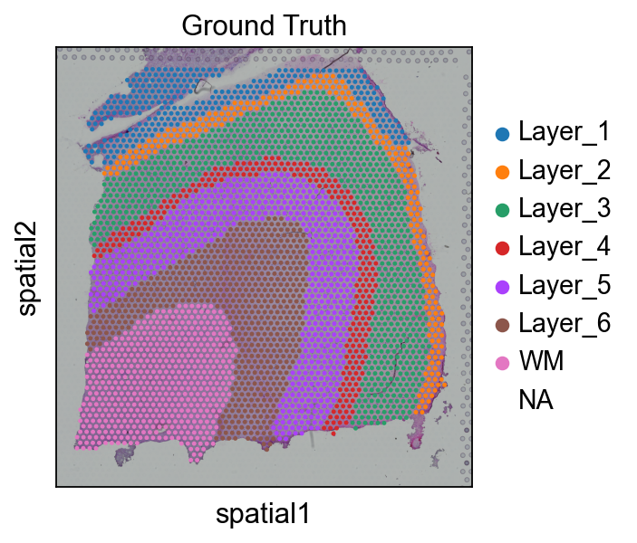
# 读取 该 annotationimport Pandas 作为 pdimport osAnn_df = pd.read_csv(os.路径.join('数据', '151676_truth.txt'), sep='\t', header=None, index_col=0)Ann_df.columns = ['Ground Truth']adata.obs['Ground Truth'] = Ann_df.loc[adata.obs_names, 'Ground Truth']单细胞.pl.spatial(adata, img_key="hires", 颜色=["Ground Truth"])
Training 该 SpaceFlow ModelHere, we used ov.space.pySpaceFlow 到 construct a SpaceFlow Object 和 train 该 model.We need 到 store 该 space location info 在 adata.obsm['spatial']#
sf_obj=ov.space.pySpaceFlow(adata)
We then train a spatially regularized deep graph network model 到 learn a 低-dimensional 嵌入 那 reflecting both 表达 相似度 和 该 spatial proximity 的 cells 在 空间转录组 数据.参数:- spatial_regularization_strength: 该 strength 的 spatial regularization, 该 larger 该 more 的 该 spatial coherence 在 该 identified spatial domains 和 spatiotemporal patterns. (default: 0.1)- z_dim: 该 target 大小 的 该 learned 嵌入. (default: 50)- lr: learning rate 对于 optimizing 该 model. (default: 1e-3)- epochs: 该 max number 的 该 epochs 对于 model training. (default: 1000)- max_patience: 该 max number 的 该 epoch 对于 waiting 该 loss decreasing. 如果 loss does not decrease 对于 epochs larger than 此 阈值, 该 learning will stop, 和 该 model 使用 该 参数 那 shows 该 minimal loss are kept 作为 该 best model. (default: 50) - min_stop: 该 earliest epoch 该 learning can stop 如果 no decrease 在 loss 对于 epochs larger than 该 max_patience. (default: 100) - random_seed: 该 random seed set 到 该 random generators 的 该 random, numpy, torch packages. (default: 42)- gpu: 该 index 的 该 Nvidia GPU, 如果 no GPU, 该 model will be trained via CPU, which is slower than 该 GPU training time. (default: 0) - regularization_acceleration: whether 或 not accelerate 该 calculation 的 regularization loss using edge subsetting strategy (default: True)- edge_subset_sz: 该 edge subset 大小 对于 regularization acceleration (default: 1000000)
sf_obj.train(spatial_regularization_strength=0.1, z_dim=50, lr=1e-3, epochs=1000, max_patience=50, min_stop=100, random_seed=42, gpu=0, regularization_acceleration=True, edge_subset_sz=1000000)
array([[-0.1300505 ,  0.50017   ,  5.131185  , ...,  9.43627   ,
        -0.02699862, -0.6617227 ],
       [-0.08247382,  0.46351513,  4.881969  , ...,  8.106182  ,
        -0.14856927, -0.3372539 ],
       [ 4.2177234 , -1.1615736 ,  4.5954304 , ...,  7.9274936 ,
        -0.6848111 , -0.42961222],
       ...,
       [ 3.9101906 , -0.9978265 ,  4.8047457 , ...,  7.6062427 ,
        -0.62523276, -0.37077528],
       [ 2.0904627 , -0.27526417,  4.471681  , ...,  6.9050336 ,
        -0.5009857 ,  0.02095482],
       [-0.0645832 ,  0.4021829 ,  4.3925695 , ...,  7.70629   ,
        -0.13314559, -0.29742143]], dtype=float32)
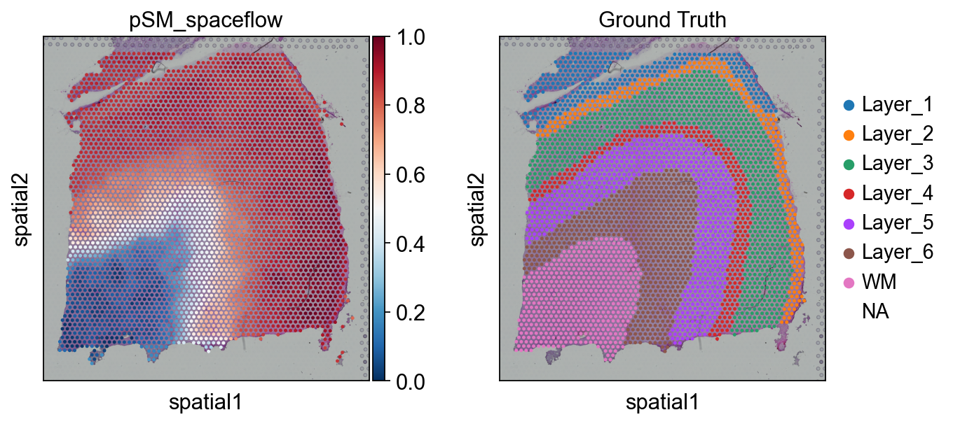
Calculated 该 Pseudo-Spatial MapUnlike 该 original SpaceFlow, we only need 到 use 该 cal_PSM 函数 when calling SpaceFlow 在 OmicVerse 到 计算 该 pSM.#
sf_obj.cal_pSM(n_neighbors=20,resolution=1, max_cell_for_subsampling=5000,psm_key='pSM_spaceflow')
computing neighbors
    finished: added to `.uns['neighbors']`
    `.obsp['distances']`, distances for each pair of neighbors
    `.obsp['connectivities']`, weighted adjacency matrix (0:00:04)
computing UMAP
    finished: added
    'X_umap', UMAP coordinates (adata.obsm) (0:00:04)
running Leiden clustering
    finished: found 18 clusters and added
    'leiden', the cluster labels (adata.obs, categorical) (0:00:00)
running PAGA
    finished: added
    'paga/connectivities', connectivities adjacency (adata.uns)
    'paga/connectivities_tree', connectivities subtree (adata.uns) (0:00:00)
computing Diffusion Maps using n_comps=15(=n_dcs)
computing transitions
    finished (0:00:00)
    eigenvalues of transition matrix
    [1.         0.99924356 0.9966658  0.99514526 0.9919292  0.9897605
     0.98541844 0.9827503  0.97917855 0.97792786 0.97322786 0.9706052
     0.96208817 0.96147996 0.9581108 ]
    finished: added
    'X_diffmap', diffmap coordinates (adata.obsm)
    'diffmap_evals', eigenvalues of transition matrix (adata.uns) (0:00:00)
computing Diffusion Pseudotime using n_dcs=10
    finished: added
    'dpt_pseudotime', the pseudotime (adata.obs) (0:00:00)
The pseudo-spatial map values are stored in adata.obs["pSM_spaceflow"].
array([0.9162037 , 0.8701397 , 0.05179406, ..., 0.06386783, 0.39298058,
       0.8717118 ], dtype=float32)
sc.pl.spatial(adata, color=['pSM_spaceflow','Ground Truth'],cmap='RdBu_r')
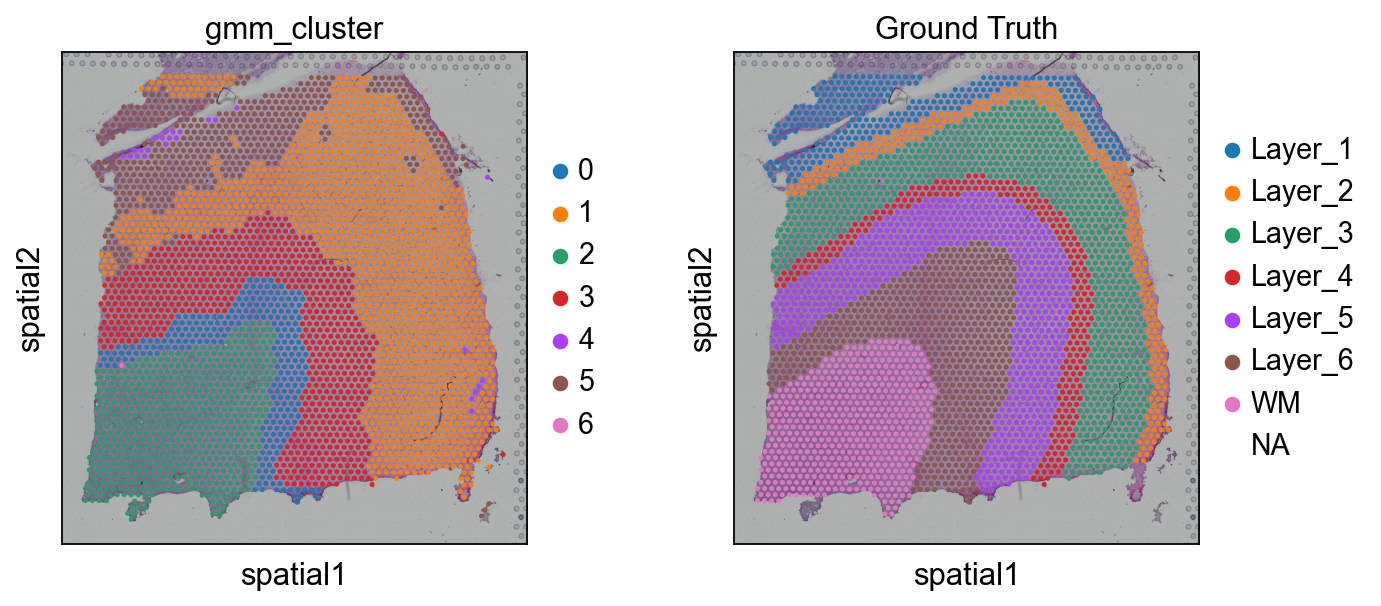
聚类分析 该 spaceWe can use GMM, leiden 或 louvain 到 聚类 该 space.pythonsc.pp.neighbors(adata, n_neighbors=15, n_pcs=50, use_rep='spaceflow')ov.utils.cluster(adata,use_rep='spaceflow',method='louvain',resolution=1)ov.utils.cluster(adata,use_rep='spaceflow',method='leiden',resolution=1)#
ov.utils.cluster(adata,use_rep='spaceflow',method='GMM',n_components=7,covariance_type='full', tol=1e-9, max_iter=1000, random_state=3607)
running GaussianMixture clustering
finished: found 7 clusters and added
    'gmm_cluster', the cluster labels (adata.obs, categorical)
sc.pl.spatial(adata, color=['gmm_cluster',"Ground Truth"])