基于参考scRNA-seq的Bulk反卷积

细胞类型反卷积是一种计算框架，旨在推断bulk异质组织中细胞群体的组成。Bulk反卷积方法可分为基于线性回归的方法、基于富集的方法、基于非线性深度学习的方法及其他方法。

这里，我们提供Bayesprime和scaden，通过类omicverse.bulk.Deconvolution使用scRNA-seq作为参考来推断细胞类型组成。用户可以在Python环境中通过omicverse非常轻松地运行bulk反卷积。我们结合了InstaPrism和pybayesprime来加速计算。

%load_ext autoreload
%autoreload 2

import omicverse as ov
ov.plot_set()

🔬 Starting plot initialization...
🧬 Detecting GPU devices…
✅ Apple Silicon MPS detected
    • [MPS] Apple Silicon GPU - Metal Performance Shaders available

   ____            _     _    __                  
  / __ \____ ___  (_)___| |  / /__  _____________ 
 / / / / __ `__ \/ / ___/ | / / _ \/ ___/ ___/ _ \ 
/ /_/ / / / / / / / /__ | |/ /  __/ /  (__  )  __/ 
\____/_/ /_/ /_/_/\___/ |___/\___/_/  /____/\___/                                              

🔖 Version: 1.7.8rc1   📚 Tutorials: https://omicverse.readthedocs.io/
✅ plot_set complete.

1. 数据准备

为了展示我们集成的bayesprime和scaden工具的准确性，本教程使用COVID-19的bulk RNA-seq数据。

• Bulk RNA-seq：我们可以通过GSE152418获取COVID-19的bulk RNA-seq数据，其中包括17名健康对照、16名COVID-19患者和1名COVID-19康复期患者。

• scRNA-seq：我们可以直接从cellxgene获取scRNA-seq参考数据，其中包括healthy和COVID组，帮助我们了解细胞类型组成。

此外，您也可以直接从figshare下载预处理好的数据（bulk rna-seq和scRNA-seq）。

bulk_ad=ov.datasets.decov_bulk_covid_bulk()
bulk_ad

🧬 Loading COVID-19 PBMC bulk data
🔍 Downloading data to ./data/COVID_PBMC_bulk.h5ad
✅ Download completed
 Loading data from ./data/COVID_PBMC_bulk.h5ad
✅ Successfully loaded: 34 cells × 60683 genes

AnnData object with n_obs × n_vars = 34 × 60683
    obs: 'days_post_symptom_onset', 'gender', 'disease_state', 'severity', 'location', 'source'

注意

“obs字段可以留空。如果您有bulk RNA-seq矩阵，可以使用ov.AnnData(count)将其转换为AnnData格式。只需确保obs包含样本名称，var包含基因名称。”

single_ad_ref=ov.datasets.decov_bulk_covid_single()
single_ad_ref

🧬 Loading COVID-19 PBMC single-cell data
🔍 Downloading data to ./data/COVID_PBMC_single.h5ad
⚠️ File ./data/COVID_PBMC_single.h5ad already exists
 Loading data from ./data/COVID_PBMC_single.h5ad
✅ Successfully loaded: 10000 cells × 24505 genes

AnnData object with n_obs × n_vars = 10000 × 24505
    obs: 'nCount_RNA', 'nFeature_RNA', 'percent.mt', 'percent.rps', 'percent.rpl', 'percent.rrna', 'nCount_SCT', 'nFeature_SCT', 'seurat_clusters', 'singler', 'cell.type.fine', 'cell.type.coarse', 'IFN1', 'HLA1', 'donor_id', 'DPS', 'DTF', 'Admission', 'Ventilated', 'tissue_ontology_term_id', 'assay_ontology_term_id', 'disease_ontology_term_id', 'cell_type_ontology_term_id', 'development_stage_ontology_term_id', 'self_reported_ethnicity_ontology_term_id', 'sex_ontology_term_id', 'is_primary_data', 'suspension_type', 'tissue_type', 'cell_type', 'assay', 'disease', 'sex', 'tissue', 'self_reported_ethnicity', 'development_stage', 'observation_joinid'
    var: 'feature_is_filtered', 'feature_name', 'feature_reference', 'feature_biotype', 'feature_length', 'feature_type'
    uns: 'cell.type.coarse_colors', 'cell.type.coarse_colors_rgba', 'cell.type.fine_colors', 'cell.type.fine_colors_rgba', 'citation', 'disease_colors', 'disease_colors_rgba', 'organism', 'organism_ontology_term_id', 'schema_reference', 'schema_version', 'title'
    obsm: 'X_pca', 'X_umap'
    layers: 'lognorm', 'recover_counts'

注意

“需要注意的是，我们的数据均为原始计数。如果您的单细胞数据经过了log1p转换，请使用omicverse.pp.recover_counts函数恢复原始表达矩阵。”

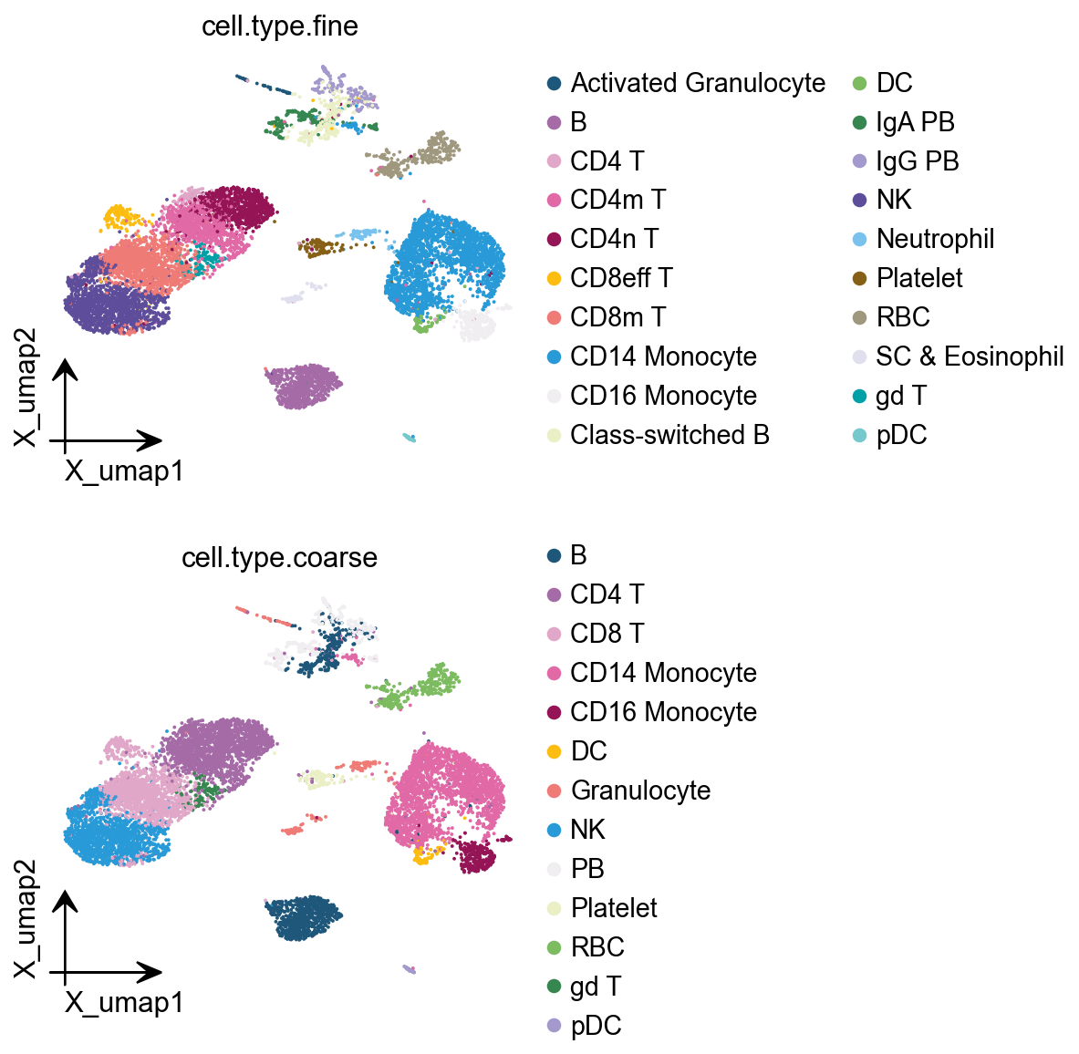
bayesprime supports simultaneous input of major and minor cell types for deconvolution. In our single-cell data, major cell types are stored in single_ad_ref.obs[‘cell.type.coarse’], while minor cell types reside in single_ad_ref.obs[‘cell.type.fine’]. while the grouping labels are stored in single_ad_ref.obs[‘disease’].

ov.pl.embedding(
    single_ad_ref,
    basis='X_umap',
    color=['cell.type.fine','cell.type.coarse'],
    ncols=1
)

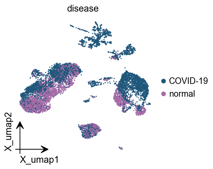
ov.pl.embedding(
    single_ad_ref,
    basis='X_umap',
    color='disease'
)

我们可以使用堆叠条形图来观察不同组间细胞比例的分布。

fig,ax=ov.plt.subplots(figsize = (1.5,3))
ov.pl.cellproportion(
    adata=single_ad_ref,
    celltype_clusters='cell.type.coarse',
    groupby='disease',legend=True,ax=ax
)

2. 运行bayesprime

在omicverse中，所有反卷积运行均通过同一个类执行。这意味着如果未来添加新方法，只需修改method参数，极大地方便了未来的基准测试。

我们首先需要定义输入的bulk RNA-seq矩阵和参考scRNA-seq矩阵。

deconv_obj=ov.bulk.Deconvolution(
    adata_bulk=bulk_ad,
    adata_single=single_ad_ref,
    max_single_cells=10000,
    celltype_key='cell.type.coarse',
    cellstate_key='cell.type.fine',
)

......single-cell reference built finished
CUDA not available, using MPS backend instead.

注意

“celltype_key和cellstate_key可以设置为相同的值。该参数仅在Bayesprime方法中使用；其他方法不涉及次细胞类型。”

res=deconv_obj.deconvolution(
    method='bayesprism',n_cores=8,fast_mode=True
)

number of cells in each cell state
No tumor reference is speficied. Reference cell types are treated equally.
Number of outlier genes filtered from mixture = 5
Aligning reference and mixture...
Normalizing reference...
============================================================
FAST MODE: Using fixed-point iteration (50-500x faster)
Note: Results are approximate (correlation >0.99 with Gibbs)
============================================================
Fast deconvolution (fixed-point iteration)...
Note: 50-500x faster but approximate results (no update_gibbs)
Run fast deconvolution using fixed-point iteration (n_iter=100)...
Note: This is 50-500x faster but provides approximate results.
Fixed-point iteration 0: max_diff = 0.021858
  Fixed-point iteration 10: max_diff = 0.012418
  Fixed-point iteration 20: max_diff = 0.003776
  Fixed-point iteration 30: max_diff = 0.001679
  Fixed-point iteration 40: max_diff = 0.001075
  Fixed-point iteration 50: max_diff = 0.000761
  Fixed-point iteration 60: max_diff = 0.000556
  Fixed-point iteration 70: max_diff = 0.000408
  Fixed-point iteration 80: max_diff = 0.000300
  Fixed-point iteration 90: max_diff = 0.000263

Completed in 29.16 seconds
  Samples: 34
  Converged: 0/34 (0.0%)
  Average iterations: 100.0
  Time per sample: 857.66 ms
Merging cell states to cell types...

注意

需要注意的是，当我们将fast_mode参数设置为True时，实际上是在调用InstaPrime。事实上，两者的相似度高达0.99。如果您希望调用BayesPrime，只需将fast_mode=False即可。

res=res[single_ad_ref.obs['cell.type.coarse'].cat.categories]
res.head()

	B	CD4 T	CD8 T	CD14 Monocyte	CD16 Monocyte	DC	Granulocyte	NK	PB	Platelet	RBC	gd T	pDC
S145_nCOV001_C	0.007152	0.045643	0.028839	0.350588	0.358540	0.063780	0.005991	0.102774	0.003153	0.019414	2.157114e-05	0.000909	0.013197
S147_nCoV001EUHM-Draw-1	0.042290	0.064573	0.145169	0.207204	0.209637	0.064921	0.014626	0.176877	0.046780	0.014637	1.785132e-10	0.003598	0.009689
S149_nCoV002EUHM-Draw-2	0.044652	0.002136	0.026601	0.435803	0.268785	0.032620	0.017837	0.083378	0.048856	0.034941	1.004674e-09	0.000243	0.004149
S150_nCoV003EUHM-Draw-1	0.016705	0.004011	0.105450	0.345644	0.154792	0.024709	0.012880	0.160400	0.152966	0.018139	5.689293e-04	0.000129	0.003605
S151_nCoV004EUHM-Draw-1	0.029047	0.000164	0.037455	0.610666	0.127016	0.009614	0.009160	0.023490	0.087138	0.062375	2.029203e-03	0.000016	0.001830

为了保持单细胞细胞类型颜色表示的一致性，我们需要重新定义color_dict。

color_dict=dict(zip(
    single_ad_ref.obs['cell.type.coarse'].cat.categories,
    single_ad_ref.uns['cell.type.coarse_colors']
))

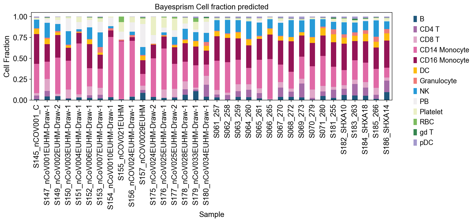
ax = res.plot(kind='bar', stacked=True, figsize=(12, 3),color=color_dict)
ax.set_xlabel('Sample')
ax.set_ylabel('Cell Fraction')
#ax.set_xticklabels([])
ax.set_title('Bayesprism Cell fraction predicted')
ov.plt.legend(bbox_to_anchor=(1.05, 1),ncol=1,)
ov.plt.show()

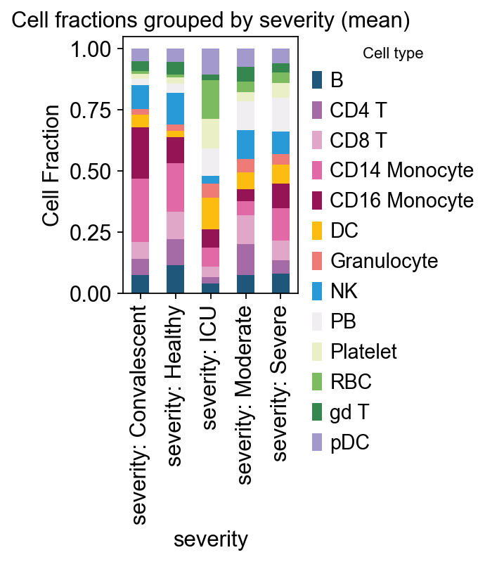
# example: severity
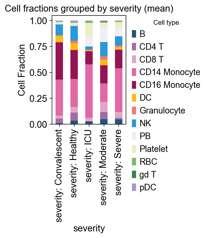
ov.pl.plot_grouped_fractions(
    res, bulk_ad.obs, group_key='severity',
    color_dict=color_dict, agg='mean', normalize=True,
    figsize=(2,3)
)

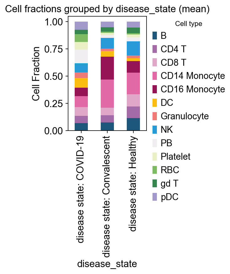
# example: disease_state
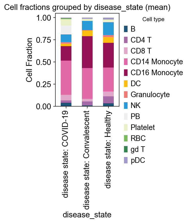
ov.pl.plot_grouped_fractions(
    res, bulk_ad.obs, group_key='disease_state', 
    color_dict=color_dict, agg='mean', normalize=True,
    figsize=(2,3)
)

<Axes: title={'center': 'Cell fractions grouped by disease_state (mean)'}, xlabel='disease_state', ylabel='Cell Fraction'>

3. 运行Scaden

Scaden是一种用于bulk RNA-seq细胞类型反卷积的工具，它使用基于scRNA-seq数据集模拟的人工bulk数据训练的深度神经网络集成。

与BayesPrime类似，运行scaden时我们也使用相同的反卷积类。

deconv_obj=ov.bulk.Deconvolution(
    adata_bulk=bulk_ad,
    adata_single=single_ad_ref,
    max_single_cells=10000,
    celltype_key='cell.type.coarse',
    cellstate_key='cell.type.fine',
    gpu='mps'
)

......single-cell reference built finished
Using Apple Metal Performance Shaders (MPS) backend.

注意

由于Scaden是基于深度学习的方法，我们需要配置运行torch的设备，包括Nvidia的CUDA、Apple的MPS，或直接在CPU上运行。

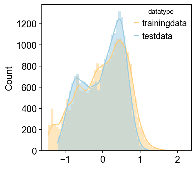
与BayesPrime相比，scaden需要配置更多参数，包括scaler、scale和datatype。scaler决定了我们如何对单细胞reads生成的伪bulk和实际bulk数据进行归一化。scale则表示是否需要在将数据输入scaler之前对其进行最小-最大归一化。

res2=deconv_obj.deconvolution(
    method='scaden',scaler='ss',scale=True,datatype='counts',
    pseudobulk_size=2000,
)

Reading single-cell dataset, this may take 1 min
Reading dataset is done
Normalizing raw single cell data with scanpy.pp.normalize_total
Generating cell fractions using Dirichlet distribution without prior info (actually random)
RANDOM cell fractions is generated
You set sparse as True, some cell's fraction will be zero, the probability is 0.5
Sampling cells to compose pseudo-bulk data
Sampling is done
Reading training data
Reading is done
Reading test data
Reading test data is done
Using counts data to train model
Cutting variance...
Finding intersected genes...
Intersected gene number is  23734
Scaling...
Using standard scaler...
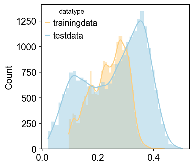
training data shape is  (2000, 23734) 
test data shape is  (34, 23734)
train model256 now
train model512 now
train model1024 now
Training of Scaden is done

注意

需要特别注意的是，虽然scaden的原始实现支持TPM、RPKM等指标，但我们强烈建议使用原始计数数据以确保算法的一致性。

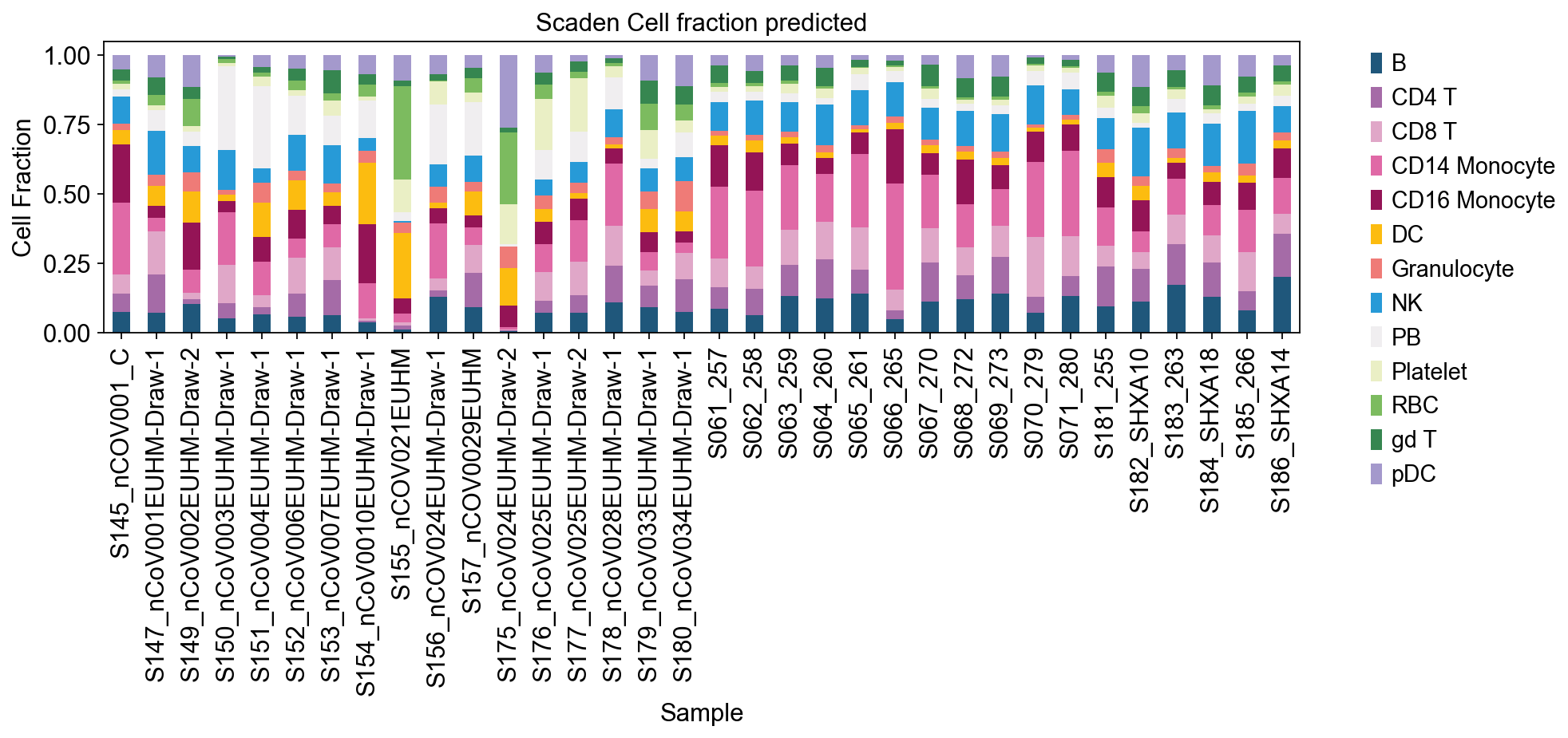
res2=res2[single_ad_ref.obs['cell.type.coarse'].cat.categories]

ax = res2.plot(kind='bar', stacked=True, figsize=(12, 3),color=color_dict)
ax.set_xlabel('Sample')
ax.set_ylabel('Cell Fraction')
#ax.set_xticklabels([])
ax.set_title('Scaden Cell fraction predicted')
ov.plt.legend(bbox_to_anchor=(1.05, 1),ncol=1,)
ov.plt.show()

# example: severity
ov.pl.plot_grouped_fractions(
    res2, bulk_ad.obs, group_key='severity',
    color_dict=color_dict, agg='mean', normalize=True,
    figsize=(2,3)
)

# example: disease_state
ov.pl.plot_grouped_fractions(
    res2, bulk_ad.obs, group_key='disease_state', 
    color_dict=color_dict, agg='mean', normalize=True,
    figsize=(2,3)
)

<Axes: title={'center': 'Cell fractions grouped by disease_state (mean)'}, xlabel='disease_state', ylabel='Cell Fraction'>