单细胞聚类和注释#
聚类是单细胞分析中的基本步骤,用于将相似的细胞分组在一起。在本教程中,我们将演示如何在OmicVerse中执行聚类和细胞类型注释。
import omicverse as ovimport scanpy as scimport scvelo as scvov.plot_set(font_path='Arial')
🔬 Starting plot initialization...
Using already downloaded Arial font from: /tmp/omicverse_arial.ttf
Registered as: Arial
🧬 Detecting CUDA devices…
✅ [GPU 0] NVIDIA A40
    • Total memory: 44.3 GB
    • Compute capability: 8.6

   ____            _     _    __
  / __ \____ ___  (_)___| |  / /__  _____________
 / / / / __ `__ \/ / ___/ | / / _ \/ ___/ ___/ _ \
/ /_/ / / / / / / / /__ | |/ /  __/ /  (__  )  __/
\____/_/ /_/ /_/_/\___/ |___/\___/_/  /____/\___/

🔖 Version: 1.7.2rc1   📚 Tutorials: https://omicverse.readthedocs.io/
✅ plot_set complete.
import scvelo as scvadata=scv.datasets.dentategyrus()adata
AnnData object with n_obs × n_vars = 2930 × 13913
    obs: 'clusters', 'age(days)', 'clusters_enlarged'
    uns: 'clusters_colors'
    obsm: 'X_umap'
    layers: 'ambiguous', 'spliced', 'unspliced'
adata=ov.pp.preprocess(adata,mode='shiftlog|pearson',n_HVGs=3000,)adata.raw = adataadata = adata[:, adata.var.highly_variable_features]ov.pp.scale(adata)ov.pp.pca(adata,layer='scaled',n_pcs=50)
Begin robust gene identification
After filtration, 13264/13913 genes are kept.     Among 13264 genes, 13189 genes are robust.
End of robust gene identification.
Begin size normalization: shiftlog and HVGs selection pearson
normalizing counts per cell
The following highly-expressed genes are not considered during normalization factor computation:
['Hba-a1', 'Malat1', 'Ptgds', 'Hbb-bt']
    finished (0:00:00)
extracting highly variable genes
--> added
    'highly_variable', boolean vector (adata.var)
    'highly_variable_rank', float vector (adata.var)
    'highly_variable_nbatches', int vector (adata.var)
    'highly_variable_intersection', boolean vector (adata.var)
    'means', float vector (adata.var)
    'variances', float vector (adata.var)
    'residual_variances', float vector (adata.var)
Time to analyze data in cpu: 0.458479642868042 seconds.
End of size normalization: shiftlog and HVGs selection pearson
computing PCA
    with n_comps=50
    finished (0:00:07)
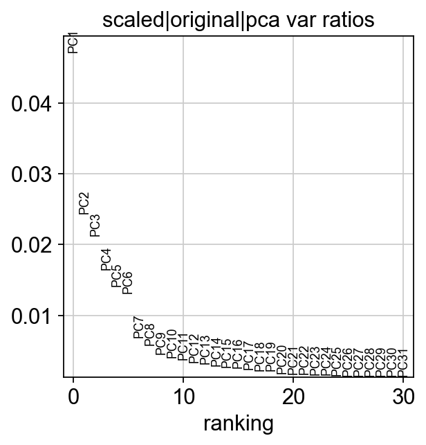
数据预处理#
首先,我们对数据进行质量控制和预处理。
ov.utils.plot_pca_variance_ratio(adata)
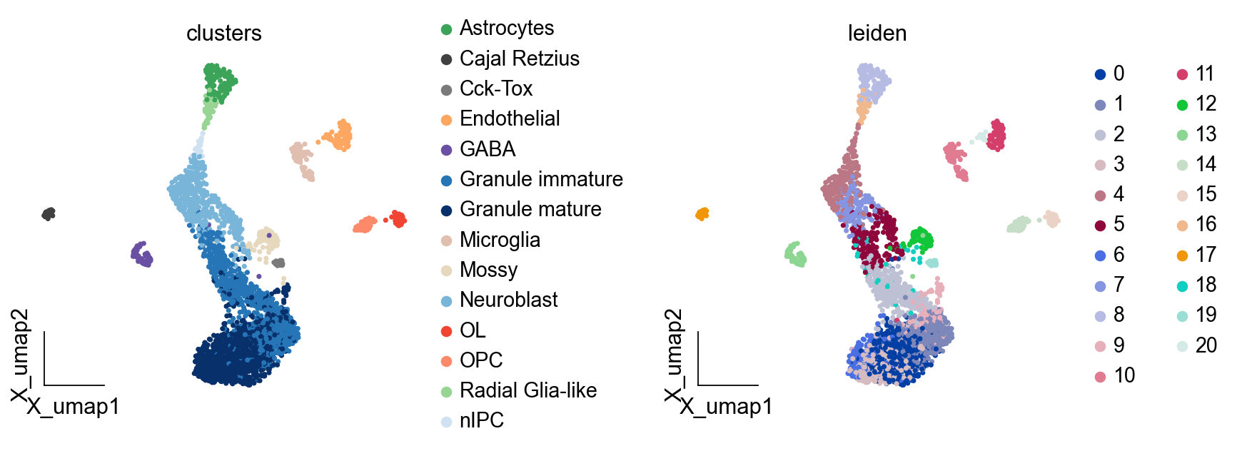
聚类方法#
OmicVerse支持多种聚类算法,包括Leiden、Louvain和其他方法。
sc.pp.neighbors(adata, n_neighbors=15, n_pcs=50, use_rep='scaled|original|X_pca')ov.utils.cluster(adata,method='leiden',resolution=1)
computing neighbors
    finished: added to `.uns['neighbors']`
    `.obsp['distances']`, distances for each pair of neighbors
    `.obsp['connectivities']`, weighted adjacency matrix (0:00:04)
running Leiden clustering
    finished: found 21 clusters and added
    'leiden', the cluster labels (adata.obs, categorical) (0:00:00)
ov.pl.embedding(adata,basis='X_umap', color=['clusters','leiden'], frameon='small',wspace=0.5)
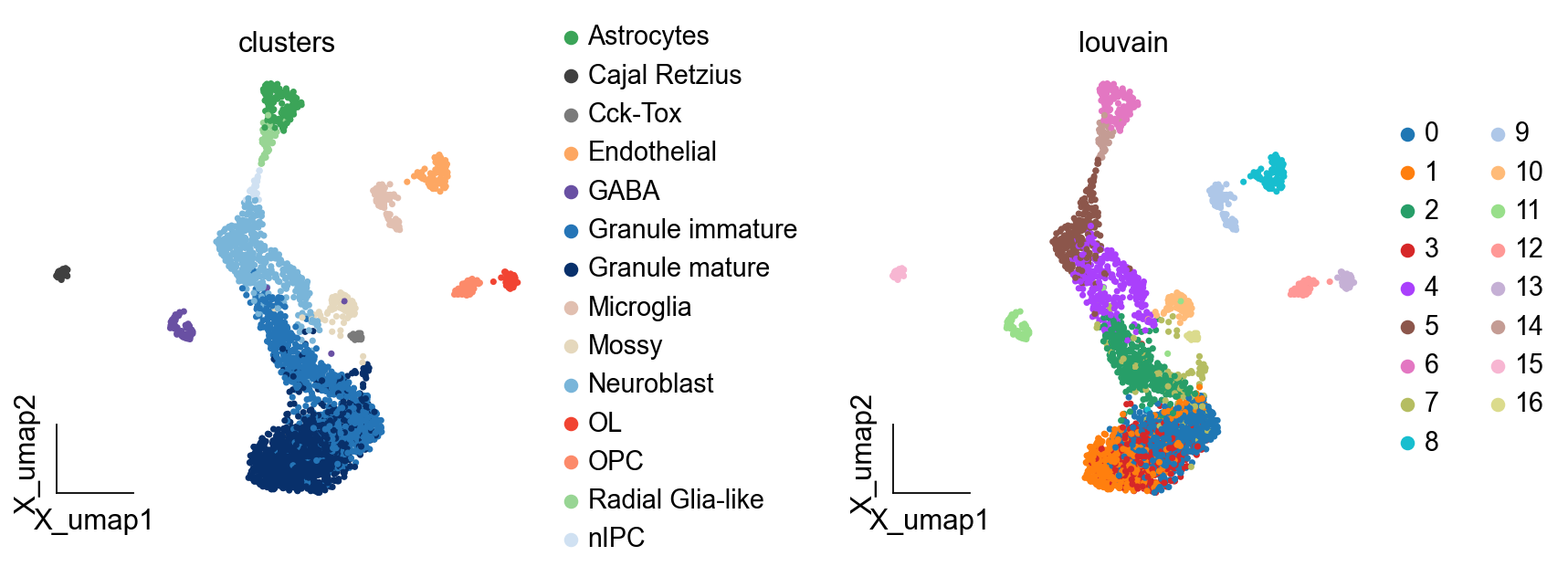
聚类参数的选择#
不同的分辨率参数会导致不同粒度的聚类。
sc.pp.neighbors(adata, n_neighbors=15, n_pcs=50, use_rep='scaled|original|X_pca')ov.utils.cluster(adata,method='louvain',resolution=1)
computing neighbors
    finished: added to `.uns['neighbors']`
    `.obsp['distances']`, distances for each pair of neighbors
    `.obsp['connectivities']`, weighted adjacency matrix (0:00:00)
running Louvain clustering
    using the "louvain" package of Traag (2017)
    finished: found 17 clusters and added
    'louvain', the cluster labels (adata.obs, categorical) (0:00:00)
ov.pl.embedding(adata,basis='X_umap', color=['clusters','louvain'], frameon='small',wspace=0.5)
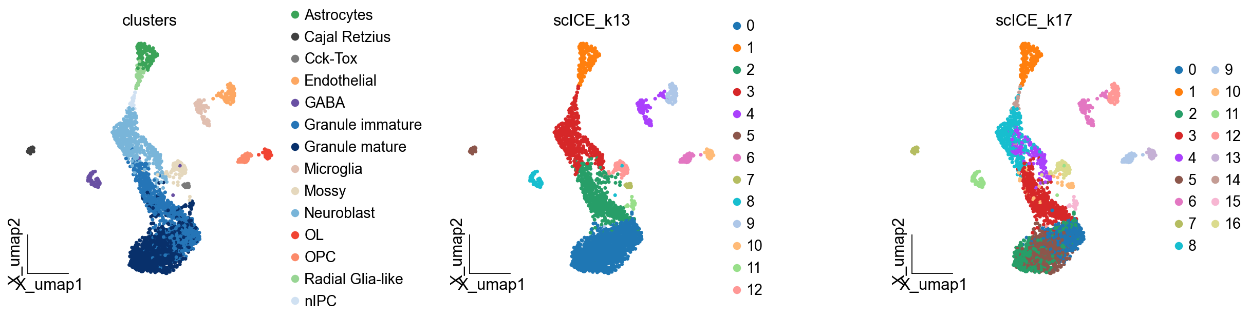
可视化聚类结果#
我们使用UMAP和tSNE等降维方法可视化聚类。
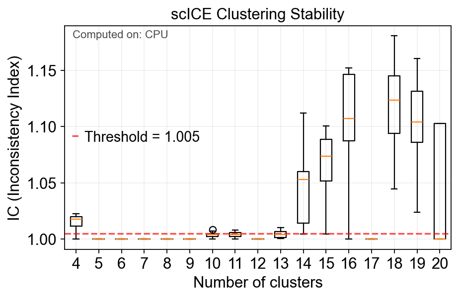
model=ov.utils.cluster( adata, method='scICE', use_rep='scaled|original|X_pca', resolution_range=(4,20), n_boot=50, n_steps=11)
🔧 Device: CPU, Parallel jobs: -1
All required Python packages are properly installed.
Building neighborhood graph...
Converting graph to igraph format...
Starting scICE clustering with CPU...
Exploring 17 cluster numbers: [4, 5, 6, 7, 8, 9, 10, 11, 12, 13, 14, 15, 16, 17, 18, 19, 20]
🚀 Using parallel processing: each thread handles one cluster number
🔧 Processing 17 cluster numbers in parallel...
Computing MEI scores...
✅ Completed scICE clustering. Found 17/17 stable solutions.
📊 Average IC score: 1.0289
🎯 Stable cluster numbers found: [4, 5, 6, 7, 8, 9, 10, 11, 12, 13, 14, 15, 16, 17, 18, 19, 20]
Added 11 stable clustering solutions to adata.obs
scICE_cluster has been added to adata.obs
fig=model.plot_ic(figsize=(6,4))
ov.pl.embedding(adata,basis='X_umap', color=['clusters','scICE_k13','scICE_k17'], frameon='small',wspace=0.5)
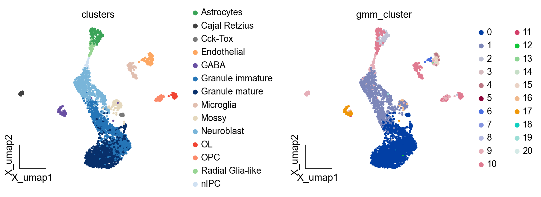
簇的表征#
一旦我们确定了簇,我们就可以通过查看不同基因的表达来表征它们。
ov.utils.cluster(adata,use_rep='scaled|original|X_pca', method='GMM',n_components=21, covariance_type='full',tol=1e-9, max_iter=1000, )
running GaussianMixture clustering
finished: found 21 clusters and added
    'gmm_cluster', the cluster labels (adata.obs, categorical)
ov.pl.embedding(adata,basis='X_umap', color=['clusters','gmm_cluster'], frameon='small',wspace=0.5)
差异表达分析#
我们进行差异表达分析来识别定义每个簇的基因。
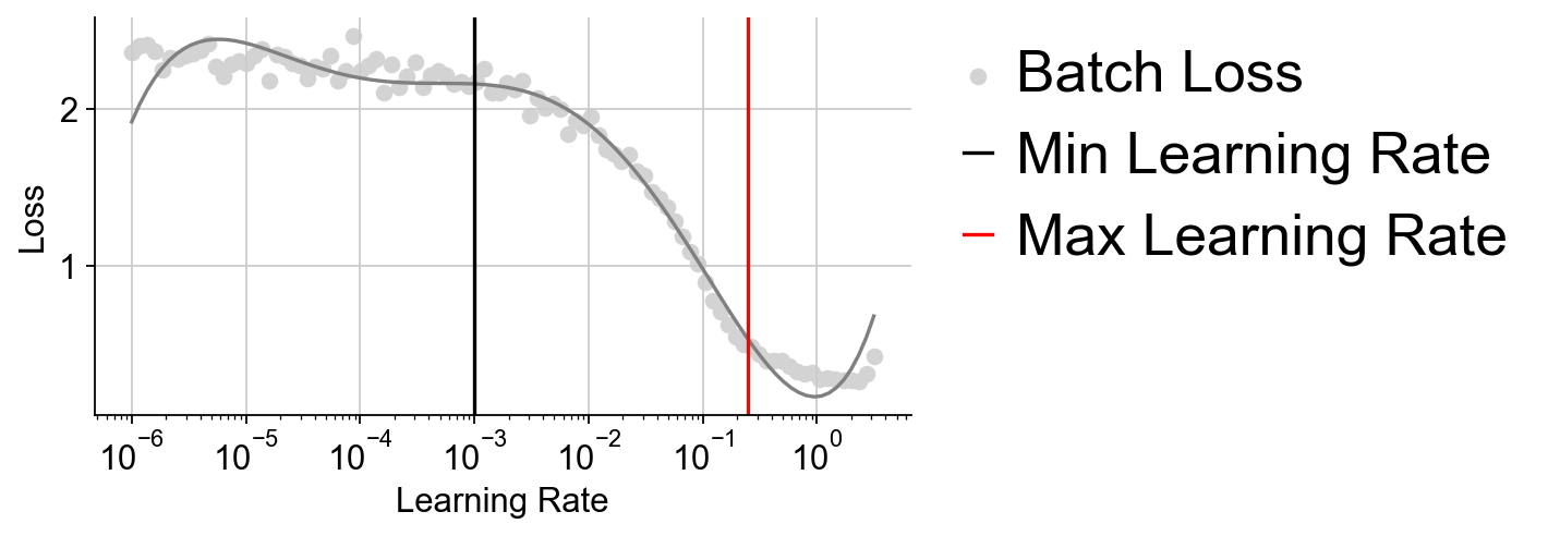
LDA_obj=ov.utils.LDA_topic(adata,feature_type='expression', highly_variable_key='highly_variable_features', layers='counts',batch_key=None,learning_rate=1e-3)
mira have been install version: 2.1.0
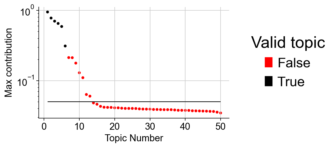
注释簇#
使用差异表达分析的结果,我们可以标记簇为特定的细胞类型。
LDA_obj.plot_topic_contributions(6)
簇的质量控制#
我们评估我们的聚类结果的质量。
LDA_obj.predicted(13)
running LDA topic predicted
finished: found 13 clusters and added
    'LDA_cluster', the cluster labels (adata.obs, categorical)
处理批次效应#
如果数据来自多个批次或样本,我们需要处理批次效应。
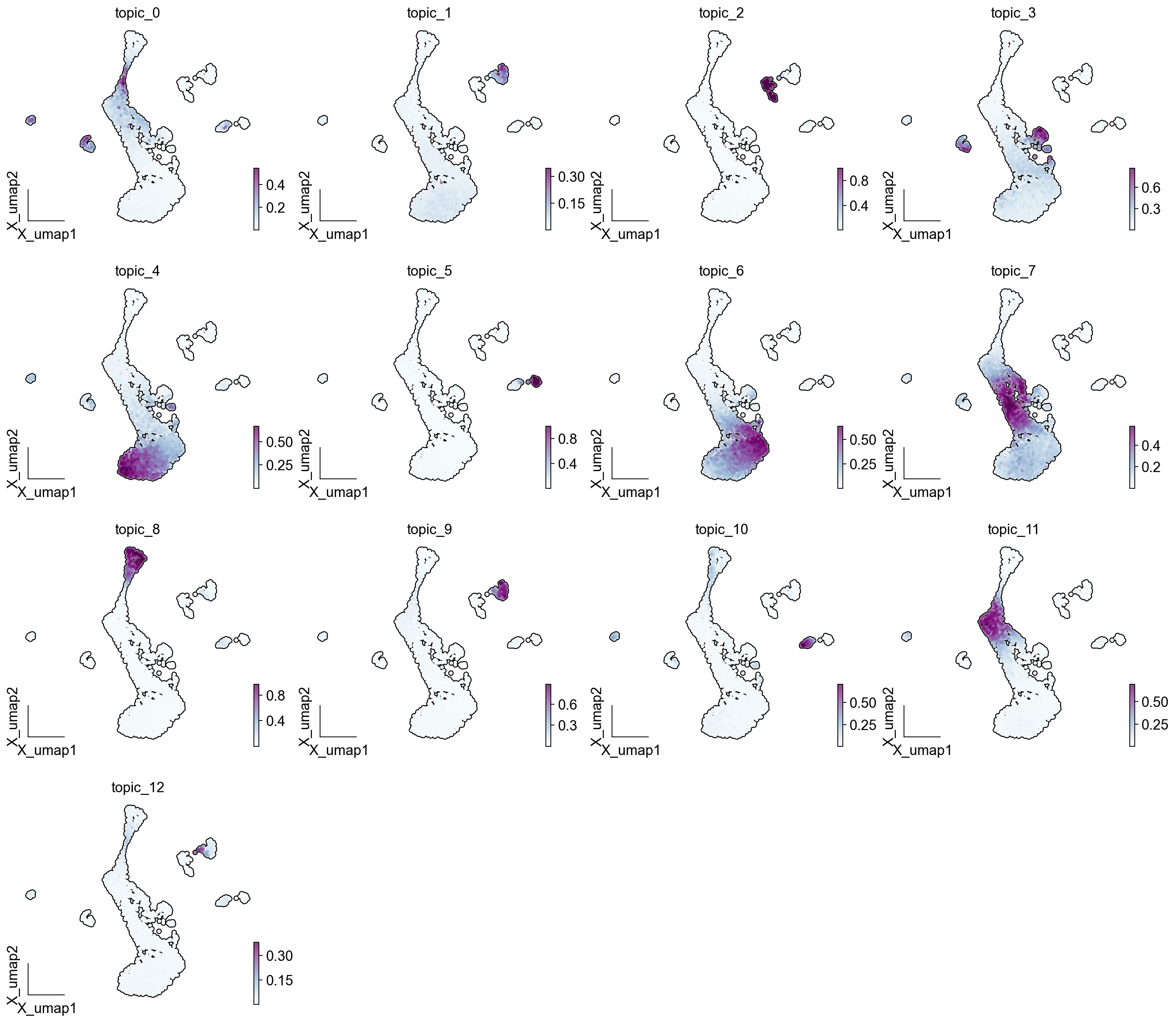
ov.plot_set()ov.pl.embedding(adata, basis='X_umap',color = LDA_obj.model.topic_cols, cmap='BuPu', ncols=4, add_outline=True, frameon='small',)
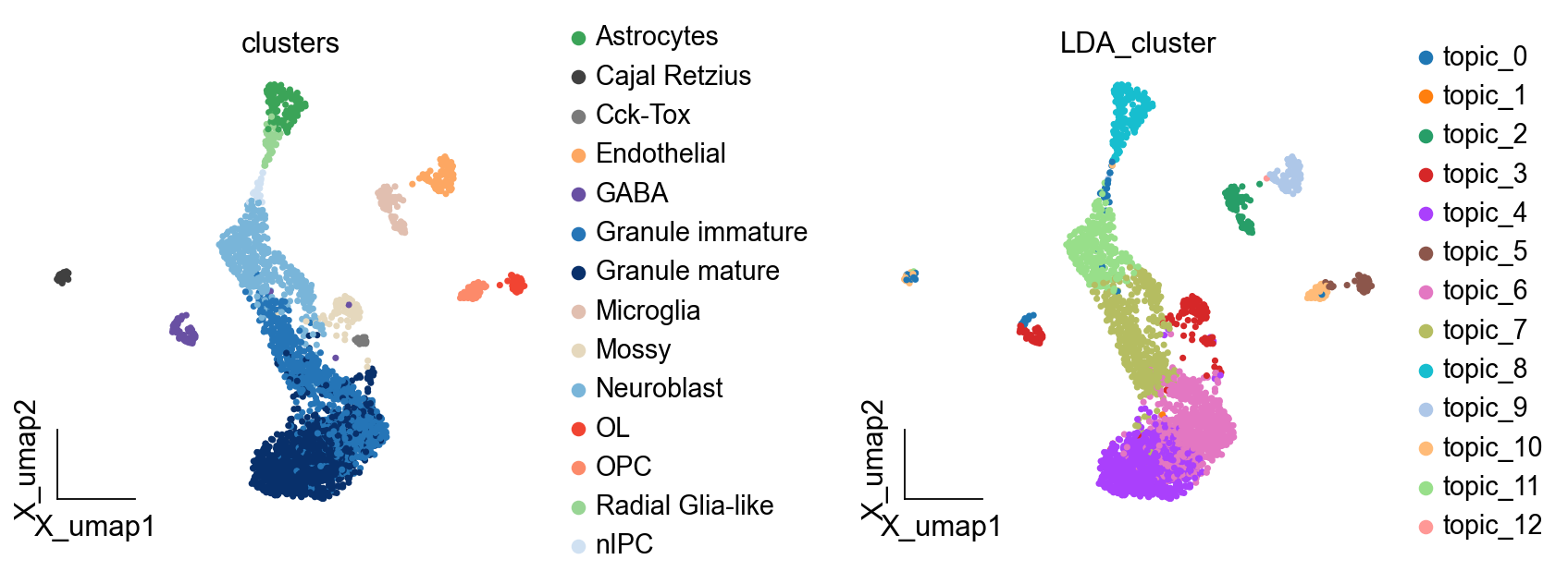
ov.pl.embedding(adata,basis='X_umap', color=['clusters','LDA_cluster'], frameon='small',wspace=0.5)
进一步的分析#
聚类完成后,我们可以进行各种下游分析。
LDA_obj.get_results_rfc(adata,use_rep='scaled|original|X_pca', LDA_threshold=0.4,num_topics=13)
running LDA topic predicted
Single Tree: 0.9617940199335548
Random Forest: 0.9883720930232558
LDA_cluster_rfc is added to adata.obs
LDA_cluster_clf is added to adata.obs
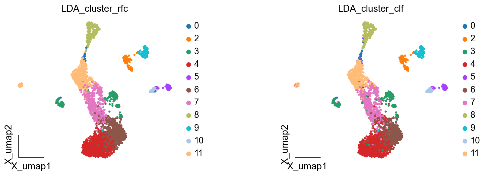
ov.pl.embedding(adata,basis='X_umap', color=['LDA_cluster_rfc','LDA_cluster_clf'], frameon='small',wspace=0.5)
总结#
在本教程中,我们学习了如何在OmicVerse中执行全面的聚类和注释分析。
adata.X.toarray()
array([[5.9377255, 0.       , 0.       , ..., 8.609415 , 0.       ,
        0.       ],
       [0.       , 0.       , 0.       , ..., 7.206903 , 0.       ,
        0.       ],
       [0.       , 0.       , 0.       , ..., 8.979355 , 0.       ,
        0.       ],
       ...,
       [0.       , 0.       , 0.       , ..., 8.287922 , 0.       ,
        0.       ],
       [0.       , 0.       , 0.       , ..., 8.657587 , 0.       ,
        0.       ],
       [0.       , 0.       , 0.       , ..., 9.004353 , 0.       ,
        5.02186  ]], dtype=float32)
# 聚类代码示例
adata = ov.datasets.pbmc3k()
ov.pp.leiden(adata, resolution=0.7)
ov.pp.umap(adata)
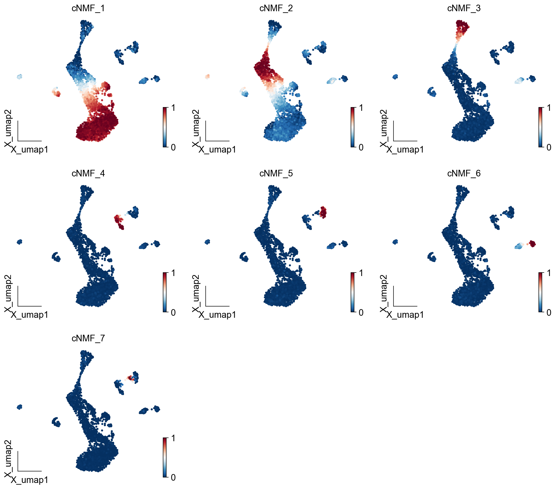
selected_K = 7density_threshold = 2.00cnmf_obj.consensus(k=selected_K, density_threshold=density_threshold, show_clustering=True, close_clustergram_fig=False)result_dict = cnmf_obj.load_results(K=selected_K, density_threshold=density_threshold)cnmf_obj.get_results(adata,result_dict)
cNMF_cluster is added to adata.obs
gene scores are added to adata.var
ov.pl.embedding(adata, basis='X_umap',color=result_dict['usage_norm'].columns, use_raw=False, ncols=3, vmin=0, vmax=1,frameon='small')
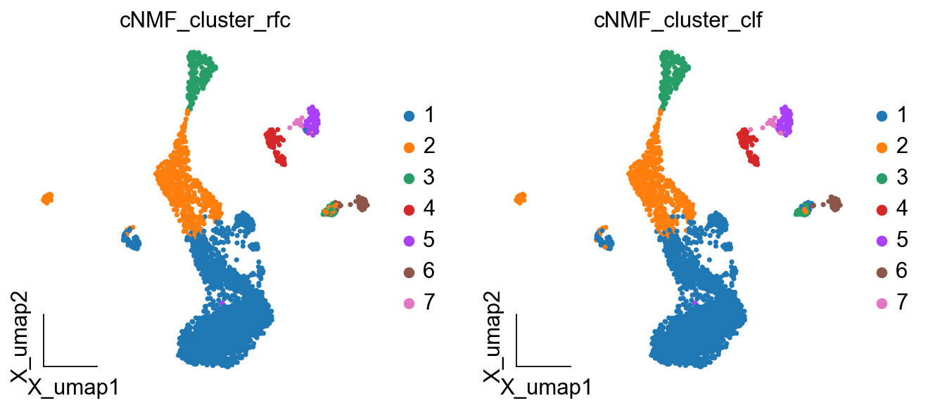
cnmf_obj.get_results_rfc(adata,result_dict, use_rep='scaled|original|X_pca', cNMF_threshold=0.5)
Single Tree: 0.9905992949471211
Random Forest: 0.9988249118683902
cNMF_cluster_rfc is added to adata.obs
cNMF_cluster_clf is added to adata.obs
# 差异表达分析
de_results = ov.single.DEG(adata, groupby='leiden', method='wilcoxon')
[<AxesSubplot: title={'center': 'cNMF_cluster_rfc'}, xlabel='X_umap1', ylabel='X_umap2'>,
 <AxesSubplot: title={'center': 'cNMF_cluster_clf'}, xlabel='X_umap1', ylabel='X_umap2'>]
交互式探索#
OmicVerse提供了工具来交互式地探索聚类结果。
from sklearn.metrics.cluster import adjusted_rand_scoreARI = adjusted_rand_score(adata.obs['clusters'], adata.obs['leiden'])print('Leiden, Adjusted rand index = %.2f' %ARI)ARI = adjusted_rand_score(adata.obs['clusters'], adata.obs['louvain'])print('Louvain, Adjusted rand index = %.2f' %ARI)ARI = adjusted_rand_score(adata.obs['clusters'], adata.obs['gmm_cluster'])print('GMM, Adjusted rand index = %.2f' %ARI)ARI = adjusted_rand_score(adata.obs['clusters'], adata.obs['LDA_cluster'])print('LDA, Adjusted rand index = %.2f' %ARI)ARI = adjusted_rand_score(adata.obs['clusters'], adata.obs['LDA_cluster_rfc'])print('LDA_rfc, Adjusted rand index = %.2f' %ARI)ARI = adjusted_rand_score(adata.obs['clusters'], adata.obs['LDA_cluster_clf'])print('LDA_clf, Adjusted rand index = %.2f' %ARI)ARI = adjusted_rand_score(adata.obs['clusters'], adata.obs['cNMF_cluster_rfc'])print('cNMF_rfc, Adjusted rand index = %.2f' %ARI)ARI = adjusted_rand_score(adata.obs['clusters'], adata.obs['cNMF_cluster_clf'])print('cNMF_clf, Adjusted rand index = %.2f' %ARI)
Leiden, Adjusted rand index = 0.36
Louvain, Adjusted rand index = 0.38
GMM, Adjusted rand index = 0.49
LDA, Adjusted rand index = 0.53
LDA_rfc, Adjusted rand index = 0.54
LDA_clf, Adjusted rand index = 0.51
LDA_rfc, Adjusted rand index = 0.41
LDA_clf, Adjusted rand index = 0.41
与其他工具的集成#
OmicVerse与其他广泛使用的工具兼容,如Seurat和Cellranger。