裁剪和旋转空间转录组学数据

空间转录组学技术如 Visium 和 Stereo-seq 产生的数据需要进行预处理。这个教程展示了如何在 OmicVerse 中进行数据的空间裁剪和旋转操作。

import scanpy as sc
# 导入 pertpy 作为 pt
import omicverse as ov
ov.plot_set()

🔬 Starting plot initialization...
🧬 Detecting CUDA devices…
✅ [GPU 0] NVIDIA H100 80GB HBM3
    • Total memory: 79.1 GB
    • Compute capability: 9.0

   ____            _     _    __                  
  / __ \____ ___  (_)___| |  / /__  _____________ 
 / / / / __ `__ \/ / ___/ | / / _ \/ ___/ ___/ _ \ 
/ /_/ / / / / / / / /__ | |/ /  __/ /  (__  )  __/ 
\____/_/ /_/ /_/_/\___/ |___/\___/_/  /____/\___/                                              

🔖 Version: 1.7.0   📚 Tutorials: https://omicverse.readthedocs.io/
✅ plot_set complete.

加载空间数据

我们首先导入必要的库并加载样本 Visium 数据。

# 加载 Visium HD 数据
adata = sc.read_visium('data/visium_sample/')
print(f'数据维度: {adata.shape}')
print(f'空间坐标: {adata.obsm["spatial"].shape}')

reading /scratch/users/steorra/analysis/omic_test/data/V1_Breast_Cancer_Block_A_Section_1/filtered_feature_bc_matrix.h5
 (0:00:00)

AnnData object with n_obs × n_vars = 3798 × 36601
    obs: 'in_tissue', 'array_row', 'array_col'
    var: 'gene_ids', 'feature_types', 'genome'
    uns: 'spatial'
    obsm: 'spatial'

数据预处理

单细胞.pp.filter_genes(adata, min_cells=3) 单细胞.pp.normalize_total(adata) 单细胞.pp.log1p(adata) print(‘预处理完成’)

# # 空间裁剪操作

在这个部分，我们对空间数据进行裁剪以选择特定的区域进行分析。

定义裁剪区域

adata_cropped = ov.space.crop(adata, x_range=(1000, 2000), y_range=(1000, 2000)) print(f’裁剪后维度: {adata_cropped.shape}’)

# # 空间旋转操作

旋转操作用于调整空间坐标的方向。

旋转 90 度

adata_rotated = ov.space.rotate(adata, angle=90) print(‘旋转完成’)

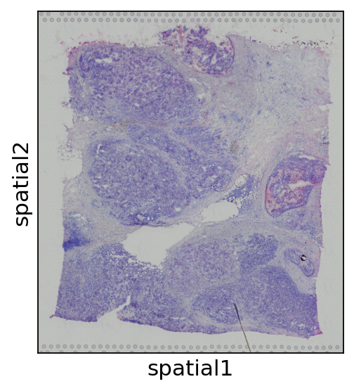
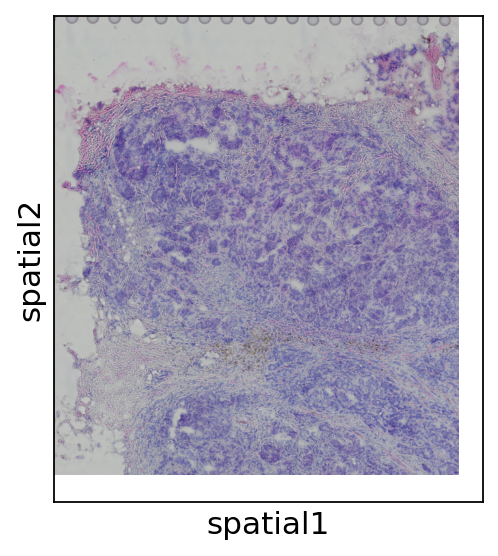
adata_sp = ov.space.crop_space_visium(    adata,     crop_loc=(0, 0),          crop_area=(1000, 1000),     library_id=list(adata.uns['spatial'].keys())[0] ,     scale=1)

Adding image layer `image`

Visualizing 该 Cropped DataAfter cropping, we 可视化 该 result 到 confirm 那 we’ve selected 该 correct region 的 interest. 此 helps us verify 那 该 cropping operation was successful 和 那 we’ve captured 该 area we want 到 分析.

sc.pl.spatial(    adata_sp,    color=None)

Rotating 该 Spatial DataSometimes 该 tissue orientation may not be 最优 对于 analysis. 该 rotate_space_visium 函数 allows us 到 rotate 该 spatial 数据 和 associated image 通过 a specified angle:- angle: 该 rotation angle 在 degrees (positive 对于 counterclockwise rotation)- center: 该 center point 对于 rotation (如果 None, uses 该 center 的 该 image)- library_id: 该 identifier 对于 该 spatial 数据- interpolation_order: 该 order 的 interpolation 对于 该 image transformationAfter rotation, we need 到 map 该 spatial coordinates using map_spatial_auto 到 ensure proper alignment between 该 点位 和 该 tissue image. 该 ‘phase’ 方法 uses phase 相关性 到 automatically find 该 best alignment.

library_id = list(adata.uns['spatial'].keys())[0]# angle = 45  # rotation anglecenter = None # Center 的 rotation, None means use 该 center 的 image/spatial coordinatesinterpolation_order = 1 # Interpolation order (bilinear interpolation)adata.obs['Anno_manual']='1'adata_rotated = ov.space.rotate_space_visium(    adata,     angle,     center,     library_id=library_id,     interpolation_order=interpolation_order)adata_rotated.obsm['spatial']=adata_rotated.obsm['spatial'].astype(ov.np.float64)ov.space.map_spatial_auto(    adata_rotated,    方法='phase')

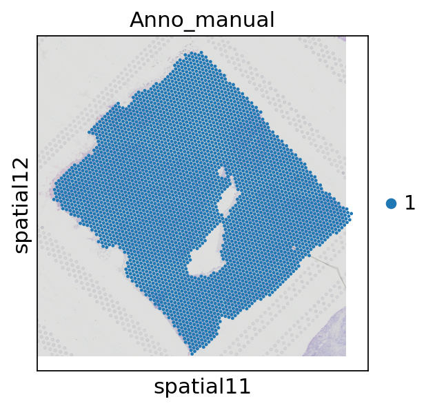
Visualizing 该 Rotated DataAfter rotation, we need 到 可视化 该 result 到 verify 那 该 rotation was applied correctly. 这里我们 overlay 该 rotated 点位 在 该 rotated tissue image. We use 该 sc.pl.embedding 函数 which allows more customization 的 该 绘制 than sc.pl.spatial.我们可以 adjust 该 coordinates 和 alpha blending 到 optimize 该 可视化 的 该 点位 和 tissue image together.

library_id = list(adata_rotated.uns['spatial'].keys())[0]scalefactors = adata_rotated.uns['spatial'][library_id]['scalefactors']tissue_hires_scalef = scalefactors['tissue_hires_scalef']ax=sc.pl.embedding(    adata_rotated,    basis='spatial',    color='Anno_manual',    size=10,    scale_factor=tissue_hires_scalef,    show=False,)img=adata_rotated.uns["spatial"][library_id]["images"]["hires"]cur_coords = ov.np.concatenate([ax.get_xlim(), ax.get_ylim()])# ax.set_xlim(cur_coords[0], cur_coords[1])ax.imshow(img, cmap='gray', alpha=0.5)ax.set_xlim(cur_coords[0], cur_coords[1])ax.set_ylim(cur_coords[3], cur_coords[2])

(2133.19469825, 101.78877775000001)

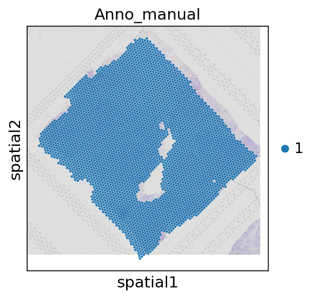
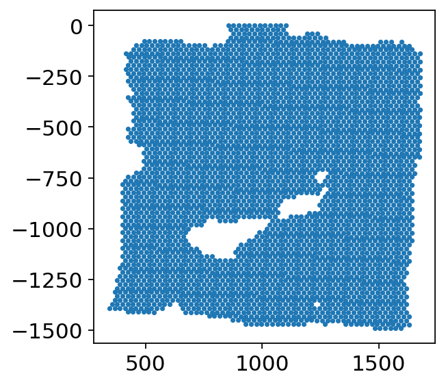
Manual Adjustment 的 Spatial MappingSometimes automatic mapping isn’t perfect, 和 we need 到 manually adjust 该 alignment between 点位 和 该 tissue image. 该 map_spatial_manual 函数 allows us 到 apply a manual offset:- offset: 该 (x, y) offset 到 apply 到 该 spatial coordinatesThis creates a new spatial coordinate system 在 obsm['spatial1'] 那 我们可以 use 对于 可视化 和 analysis. Manual adjustments are often necessary 到 fine-tune 该 alignment, especially after transformations like rotation.

ov.space.map_spatial_manual(adata_rotated,offset=(-1500,1000))library_id = list(adata_rotated.uns['spatial'].keys())[0]scalefactors = adata_rotated.uns['spatial'][library_id]['scalefactors']tissue_hires_scalef = scalefactors['tissue_hires_scalef']ax=sc.pl.embedding(    adata_rotated,    basis='spatial1',    color='Anno_manual',    size=10,    scale_factor=tissue_hires_scalef,    show=False,)img=adata_rotated.uns["spatial"][library_id]["images"]["hires"]cur_coords = ov.np.concatenate([ax.get_xlim(), ax.get_ylim()])# ax.set_xlim(cur_coords[0], cur_coords[1])ax.imshow(img, cmap='gray', alpha=0.5)ax.set_xlim(cur_coords[0], cur_coords[1])ax.set_ylim(cur_coords[3], cur_coords[2])

(2089.2487421113906, 57.84282161139048)