使用 StaVIA 进行轨迹推断#
如果在你的研究中使用了 StaVIA,请引用:
StaVIA: Spatio-Temporal Latent Embeddings and Vector field Inference for Collective Cell Migrations.
论文:<https://www.biorxiv.org/content/10.1101/2024.07.04.601964v1
Demo:https://colab.research.google.com/drive/1ssJ1tgk_QEXEotjr930UfCSmYHgSACWn?usp=sharing
%matplotlib inline

import numpy as np
import pandas as pd
import scanpy as sc
import scvelo as scv
import anndata as ad
import omicverse as ov
from anndata import AnnData
from omicverse.external import VIA

import matplotlib.pyplot as plt
ov.plot_set()
🔬 Starting plot initialization...
🧬 Detecting GPU devices…
✅ Apple Silicon MPS detected
    • [MPS] Apple Silicon GPU - Metal Performance Shaders available

   ____            _     _    __
  / __ \____ ___  (_)___| |  / /__  _____________
 / / / / __ `__ \/ / ___/ | / / _ \/ ___/ ___/ _ \
/ /_/ / / / / / / / /__ | |/ /  __/ /  (__  )  __/
\____/_/ /_/ /_/_/\___/ |___/\___/_/  /____/\___/

🔖 Version: 2.2.1rc1   📚 Tutorials: https://omicverse.readthedocs.io/
✅ plot_set complete.
加载和预处理原始教程数据#
这里保留原 StaVIA 教程使用的 dentate gyrus neurogenesis 数据集。该数据包含多个神经发生相关细胞亚群,适合展示分叉轨迹、谱系概率和基因动态。
adata = scv.datasets.dentategyrus()
adata
AnnData object with n_obs × n_vars = 2930 × 13913
    obs: 'clusters', 'age(days)', 'clusters_enlarged'
    uns: 'clusters_colors'
    obsm: 'X_umap'
    layers: 'ambiguous', 'spliced', 'unspliced'
adata = ov.pp.preprocess(adata, mode="shiftlog|pearson", n_HVGs=2000)
adata.raw = adata
adata = adata[:, adata.var.highly_variable_features].copy()
ov.pp.scale(adata)
ov.pp.pca(adata, layer="scaled", n_pcs=50)
🔍 [2026-05-23 03:40:54] Running preprocessing in 'cpu' mode...
Begin robust gene identification
    After filtration, 13264/13913 genes are kept.
    Among 13264 genes, 13189 genes are robust.
✅ Robust gene identification completed successfully.
Begin size normalization: shiftlog and HVGs selection pearson

🔍 Count Normalization:
   Target sum: 500000.0
   Exclude highly expressed: True
   Max fraction threshold: 0.2
   ⚠️ Excluding 4 highly-expressed genes from normalization computation
   Excluded genes: ['Hba-a1', 'Malat1', 'Ptgds', 'Hbb-bt']

✅ Count Normalization Completed Successfully!
   ✓ Processed: 2,930 cells × 13,189 genes
   ✓ Runtime: 0.05s

🔍 Highly Variable Genes Selection (Experimental):
   Method: pearson_residuals
   Target genes: 2,000
   Theta (overdispersion): 100
✅ Experimental HVG Selection Completed Successfully!
   ✓ Selected: 2,000 highly variable genes out of 13,189 total (15.2%)
   ✓ Results added to AnnData object:
     • 'highly_variable': Boolean vector (adata.var)
     • 'highly_variable_rank': Float vector (adata.var)
     • 'highly_variable_nbatches': Int vector (adata.var)
     • 'highly_variable_intersection': Boolean vector (adata.var)
     • 'means': Float vector (adata.var)
     • 'variances': Float vector (adata.var)
     • 'residual_variances': Float vector (adata.var)
    Time to analyze data in cpu: 0.60 seconds.
✅ Preprocessing completed successfully.
    Added:
        'highly_variable_features', boolean vector (adata.var)
        'means', float vector (adata.var)
        'variances', float vector (adata.var)
        'residual_variances', float vector (adata.var)
        'counts', raw counts layer (adata.layers)
    End of size normalization: shiftlog and HVGs selection pearson

╭─ SUMMARY: preprocess ──────────────────────────────────────────────╮
│  Duration: 0.6532s                                                 │
│  Shape:    2,930 x 13,913 -> 2,930 x 13,189                        │
│                                                                    │
│  CHANGES DETECTED                                                  │
│  ────────────────                                                  │
│  ● VAR    │ ✚ highly_variable (bool)                               │
│           │ ✚ highly_variable_features (bool)                      │
│           │ ✚ highly_variable_rank (float)                         │
│           │ ✚ means (float)                                        │
│           │ ✚ n_cells (int)                                        │
│           │ ✚ percent_cells (float)                                │
│           │ ✚ residual_variances (float)                           │
│           │ ✚ robust (bool)                                        │
│           │ ✚ variances (float)                                    │
│                                                                    │
│  ● UNS    │ ✚ REFERENCE_MANU                                       │
│           │ ✚ _ov_provenance                                       │
│           │ ✚ history_log                                          │
│           │ ✚ hvg                                                  │
│           │ ✚ log1p                                                │
│           │ ✚ status                                               │
│           │ ✚ status_args                                          │
│                                                                    │
│  ● LAYERS │ ✚ counts (sparse matrix, 2930x13189)                   │
│                                                                    │
╰────────────────────────────────────────────────────────────────────╯

╭─ SUMMARY: scale ───────────────────────────────────────────────────╮
│  Duration: 0.0232s                                                 │
│  Shape:    2,930 x 2,000 (Unchanged)                               │
│                                                                    │
│  CHANGES DETECTED                                                  │
│  ────────────────                                                  │
│  ● LAYERS │ ✚ scaled (array, 2930x2000)                            │
│                                                                    │
╰────────────────────────────────────────────────────────────────────╯
computing PCA🔍
    with n_comps=50
   🖥️ Using sklearn PCA for CPU computation
   🖥️ sklearn PCA backend: CPU computation
   📊 PCA input data type: ArrayView, shape: (2930, 2000), dtype: float64
🔧 PCA solver used: covariance_eigh
    finished✅ (3.43s)

╭─ SUMMARY: pca ─────────────────────────────────────────────────────╮
│  Duration: 3.4316s                                                 │
│  Shape:    2,930 x 2,000 (Unchanged)                               │
│                                                                    │
│  CHANGES DETECTED                                                  │
│  ────────────────                                                  │
│  ● UNS    │ ✚ pca                                                  │
│           │ └─ params: {'zero_center': True, 'use_highly_variable': Tr...│
│           │ ✚ scaled|original|cum_sum_eigenvalues                  │
│           │ ✚ scaled|original|pca_var_ratios                       │
│                                                                    │
│  ● OBSM   │ ✚ X_pca (array, 2930x50)                               │
│           │ ✚ scaled|original|X_pca (array, 2930x50)               │
│                                                                    │
╰────────────────────────────────────────────────────────────────────╯
ov.pp.neighbors(
    adata,
    use_rep="scaled|original|X_pca",
    n_neighbors=15,
    n_pcs=30,
)
ov.pp.umap(adata, min_dist=1)
🖥️ Using Scanpy CPU to calculate neighbors...

🔍 K-Nearest Neighbors Graph Construction:
   Mode: cpu
   Neighbors: 15
   Method: umap
   Metric: euclidean
   Representation: scaled|original|X_pca
   PCs used: 30
   🔍 Computing neighbor distances...
   🔍 Computing connectivity matrix...
   💡 Using UMAP-style connectivity
✓ Graph is fully connected

✅ KNN Graph Construction Completed Successfully!
   ✓ Processed: 2,930 cells with 15 neighbors each
   ✓ Results added to AnnData object:
     • 'neighbors': Neighbors metadata (adata.uns)
     • 'distances': Distance matrix (adata.obsp)
     • 'connectivities': Connectivity matrix (adata.obsp)

╭─ SUMMARY: neighbors ───────────────────────────────────────────────╮
│  Duration: 5.1772s                                                 │
│  Shape:    2,930 x 2,000 (Unchanged)                               │
│                                                                    │
│  CHANGES DETECTED                                                  │
│  ────────────────                                                  │
│  ● UNS    │ ✚ neighbors                                            │
│           │ └─ params: {'n_neighbors': 15, 'method': 'umap', 'random_s...│
│                                                                    │
│  ● OBSP   │ ✚ connectivities (sparse matrix, 2930x2930)            │
│           │ ✚ distances (sparse matrix, 2930x2930)                 │
│                                                                    │
╰────────────────────────────────────────────────────────────────────╯
🔍 [2026-05-23 03:41:03] Running UMAP in 'cpu' mode...
🖥️ Using Scanpy CPU UMAP...

🔍 UMAP Dimensionality Reduction:
   Mode: cpu
   Method: umap
   Components: 2
   Min distance: 1
{'n_neighbors': 15, 'method': 'umap', 'random_state': 0, 'metric': 'euclidean', 'use_rep': 'scaled|original|X_pca', 'n_pcs': 30}
   🔍 Computing UMAP parameters...
   🔍 Computing UMAP embedding (classic method)...
✅ UMAP Dimensionality Reduction Completed Successfully!
   ✓ Embedding shape: 2,930 cells × 2 dimensions
   ✓ Results added to AnnData object:
     • 'X_umap': UMAP coordinates (adata.obsm)
     • 'umap': UMAP parameters (adata.uns)
✅ UMAP completed successfully.

╭─ SUMMARY: umap ────────────────────────────────────────────────────╮
│  Duration: 0.4313s                                                 │
│  Shape:    2,930 x 2,000 (Unchanged)                               │
│                                                                    │
│  CHANGES DETECTED                                                  │
│  ────────────────                                                  │
│  ● UNS    │ ✚ umap                                                 │
│           │ └─ params: {'a': 0.11497568273577367, 'b': 1.9292371475038...│
│                                                                    │
╰────────────────────────────────────────────────────────────────────╯
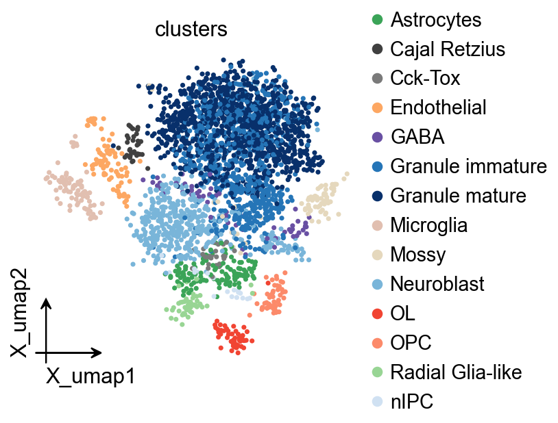
ov.pl.embedding(
    adata,
    basis="X_umap",
    color=["clusters"],
    frameon="small",
    cmap="Reds",
)
构建并运行模型#
stavia = ov.single.StaVIA(
    adata,
    use_rep="scaled|original|X_pca",
    n_comps=30,
    basis="X_umap",
    cluster_key="clusters",
    spatial_key=None,  # 空间 AnnData 可设置为 "spatial"
    time_key=None,
    sample_key=None,
    key_added="stavia",
    root="nIPC",
    knn=15,
    random_seed=4,
    memory=10,
    num_threads=1,
    n_iter_leiden=5,
    num_mcmc_simulations=200,
    edgepruning_clustering_resolution=0.15,
    cluster_graph_pruning=0.15,
    resolution_parameter=1.5,
)

stavia.fit()
v0 = stavia.model
stavia_embedding = np.asarray(adata.obsm[stavia.basis])[:, [0, 1]]
2026-05-23 03:41:05.307017	Running VIA over input data of 2930 (samples) x 30 (features)
2026-05-23 03:41:05.307110	Knngraph has 15 neighbors
2026-05-23 03:41:05.939230	Finished global pruning of 15-knn graph used for clustering at level of 0.15. Kept 43.8 % of edges.
2026-05-23 03:41:05.944493	Number of connected components used for clustergraph  is 1
2026-05-23 03:41:05.972126	Commencing community detection
2026-05-23 03:41:06.082750	Finished community detection. Found 537 clusters.
2026-05-23 03:41:06.083391	Merging 496 very small clusters (<10)
2026-05-23 03:41:06.085697	Finished detecting communities. Found 41 communities
2026-05-23 03:41:06.085792	Making cluster graph. Global cluster graph pruning level: 0.15
2026-05-23 03:41:06.088150	Graph has 1 connected components before pruning
2026-05-23 03:41:06.088985	Graph has 14 connected components after pruning
2026-05-23 03:41:06.091500	Graph has 1 connected components after reconnecting
2026-05-23 03:41:06.091661	0.0% links trimmed from local pruning relative to start
2026-05-23 03:41:06.091670	55.5% links trimmed from global pruning relative to start
initial links 346 and final_links_n 346
2026-05-23 03:41:06.092709	component number 0 out of  [0]
2026-05-23 03:41:06.106124	group root method
2026-05-23 03:41:06.106156	for component 0, the root is nIPC and ri nIPC
cluster 0 has majority Granule mature
cluster 1 has majority Granule immature
cluster 2 has majority Neuroblast
cluster 3 has majority Granule immature
cluster 4 has majority Granule immature
cluster 5 has majority Granule mature
cluster 6 has majority Granule mature
cluster 7 has majority Granule immature
cluster 8 has majority Microglia
cluster 9 has majority Neuroblast
cluster 10 has majority Astrocytes
cluster 11 has majority Mossy
cluster 12 has majority Granule mature
cluster 13 has majority Granule immature
cluster 14 has majority Granule immature
cluster 15 has majority OPC
cluster 16 has majority Astrocytes
cluster 17 has majority Neuroblast
cluster 18 has majority Granule mature
cluster 19 has majority Endothelial
cluster 20 has majority OL
cluster 21 has majority Radial Glia-like
cluster 22 has majority Granule mature
cluster 23 has majority Neuroblast
cluster 24 has majority Granule immature
cluster 25 has majority GABA
cluster 26 has majority Cck-Tox
cluster 27 has majority Neuroblast
cluster 28 has majority Cajal Retzius
cluster 29 has majority Neuroblast
cluster 30 has majority Granule mature
cluster 31 has majority GABA
cluster 32 has majority Granule mature
cluster 33 has majority nIPC
2026-05-23 03:41:06.111937	New root is 33 and majority nIPC
cluster 34 has majority Granule immature
cluster 35 has majority Granule mature
cluster 36 has majority Endothelial
cluster 37 has majority Granule mature
cluster 38 has majority Endothelial
cluster 39 has majority Granule immature
cluster 40 has majority Endothelial
2026-05-23 03:41:06.112453	Computing lazy-teleporting expected hitting times
2026-05-23 03:41:09.810906	Ended all multiprocesses, will retrieve and reshape
2026-05-23 03:41:09.824932	start computing walks with rw2 method
memory for rw2 hittings times  2. Using rw2 based pt
2026-05-23 03:41:13.053372	Identifying terminal clusters corresponding to unique lineages...
2026-05-23 03:41:13.053388	Closeness:[8, 10, 11, 15, 16, 19, 20, 21, 25, 26, 28, 31, 36, 38, 40]
2026-05-23 03:41:13.053394	Betweenness:[2, 4, 5, 6, 7, 8, 10, 11, 12, 14, 15, 16, 17, 19, 20, 22, 25, 28, 30, 31, 34, 35, 36, 38, 39]
2026-05-23 03:41:13.053399	Out Degree:[4, 5, 7, 8, 10, 11, 12, 14, 15, 16, 17, 19, 20, 21, 24, 25, 26, 28, 30, 31, 34, 36, 38, 40]
2026-05-23 03:41:13.053534	Terminal clusters corresponding to unique lineages in this component are [34, 4, 5, 36, 7, 8, 38, 11, 12, 14, 19, 25, 26, 28, 30, 31]
2026-05-23 03:41:13.053543	Calculating lineage probability at memory 10
2026-05-23 03:41:14.627760	Cluster or terminal cell fate 34 is reached 216.0 times
2026-05-23 03:41:14.656410	Cluster or terminal cell fate 4 is reached 306.0 times
2026-05-23 03:41:14.696044	Cluster or terminal cell fate 5 is reached 153.0 times
2026-05-23 03:41:14.761964	Cluster or terminal cell fate 36 is reached 1.0 times
2026-05-23 03:41:14.780277	Cluster or terminal cell fate 7 is reached 843.0 times
2026-05-23 03:41:14.808481	Cluster or terminal cell fate 8 is reached 1.0 times
2026-05-23 03:41:14.838344	Cluster or terminal cell fate 38 is reached 1.0 times
2026-05-23 03:41:14.865611	Cluster or terminal cell fate 11 is reached 36.0 times
2026-05-23 03:41:14.891106	Cluster or terminal cell fate 12 is reached 281.0 times
2026-05-23 03:41:14.917297	Cluster or terminal cell fate 14 is reached 263.0 times
2026-05-23 03:41:14.945815	Cluster or terminal cell fate 19 is reached 1.0 times
2026-05-23 03:41:14.973022	Cluster or terminal cell fate 25 is reached 33.0 times
2026-05-23 03:41:15.000335	Cluster or terminal cell fate 26 is reached 36.0 times
2026-05-23 03:41:15.028045	Cluster or terminal cell fate 28 is reached 1.0 times
2026-05-23 03:41:15.055344	Cluster or terminal cell fate 30 is reached 238.0 times
2026-05-23 03:41:15.083917	Cluster or terminal cell fate 31 is reached 33.0 times
2026-05-23 03:41:15.090085	There are (16) terminal clusters corresponding to unique lineages {34: 'Granule immature', 4: 'Granule immature', 5: 'Granule mature', 36: 'Endothelial', 7: 'Granule immature', 8: 'Microglia', 38: 'Endothelial', 11: 'Mossy', 12: 'Granule mature', 14: 'Granule immature', 19: 'Endothelial', 25: 'GABA', 26: 'Cck-Tox', 28: 'Cajal Retzius', 30: 'Granule mature', 31: 'GABA'}
2026-05-23 03:41:15.090123	Begin projection of pseudotime and lineage likelihood
2026-05-23 03:41:15.389211	Cluster graph layout based on forward biasing
2026-05-23 03:41:15.391064	Starting make edgebundle viagraph...
2026-05-23 03:41:17.531099	Make via clustergraph edgebundle
2026-05-23 03:41:17.685271	Hammer dims: Nodes shape: (41, 2) Edges shape: (154, 3)
2026-05-23 03:41:17.685579	Graph has 1 connected components before pruning
2026-05-23 03:41:17.686319	Graph has 18 connected components after pruning
2026-05-23 03:41:17.689578	Graph has 1 connected components after reconnecting
2026-05-23 03:41:17.689738	51.3% links trimmed from local pruning relative to start
2026-05-23 03:41:17.689748	53.2% links trimmed from global pruning relative to start
initial links 154 and final_links_n 75
2026-05-23 03:41:17.690758	Start making edgebundle milestone with 150 milestones...This can be recomputed with make_edgebundle_milestone()
2026-05-23 03:41:17.690770	Start finding milestones
2026-05-23 03:41:18.110668	End milestones with 150
2026-05-23 03:41:18.110752	Will use via-pseudotime for edges, otherwise consider providing a list of numeric labels (single cell level) or via_object
2026-05-23 03:41:18.113155	Recompute weights
2026-05-23 03:41:18.126492	pruning milestone graph based on recomputed weights
2026-05-23 03:41:18.127152	Graph has 1 connected components before pruning
2026-05-23 03:41:18.127428	Graph has 4 connected components after pruning
2026-05-23 03:41:18.128509	Graph has 1 connected components after reconnecting
2026-05-23 03:41:18.128922	66.4% links trimmed from global pruning relative to start
2026-05-23 03:41:18.128936	regenerate igraph on pruned edges
2026-05-23 03:41:18.132266	Setting numeric label as single cell pseudotime for coloring edges
2026-05-23 03:41:18.137103	Making smooth edges
REMEMBER TO RE-INCLUDE the PLT.SHOW HERE - COMMENTING IT OUT FOR NOW
2026-05-23 03:41:18.432596	Time elapsed 12.8 seconds
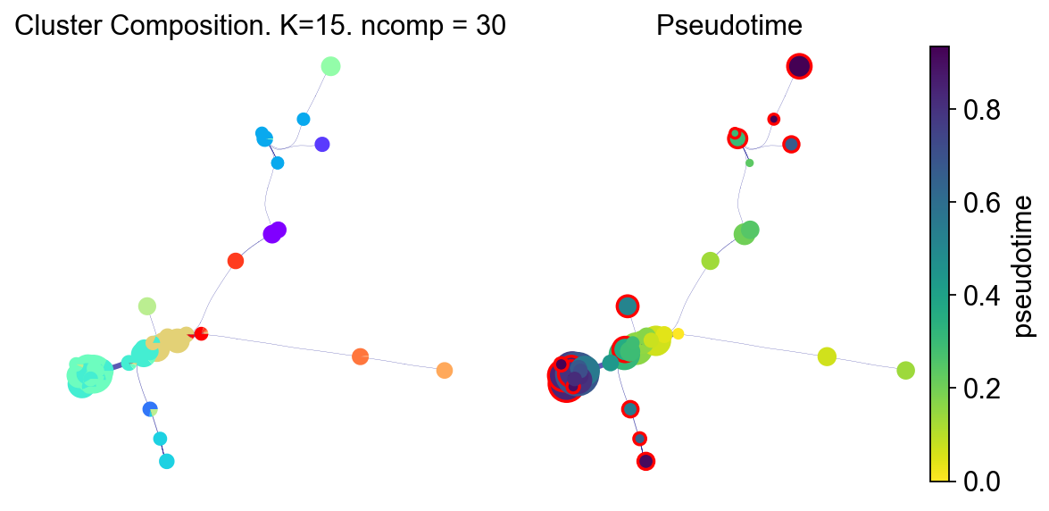
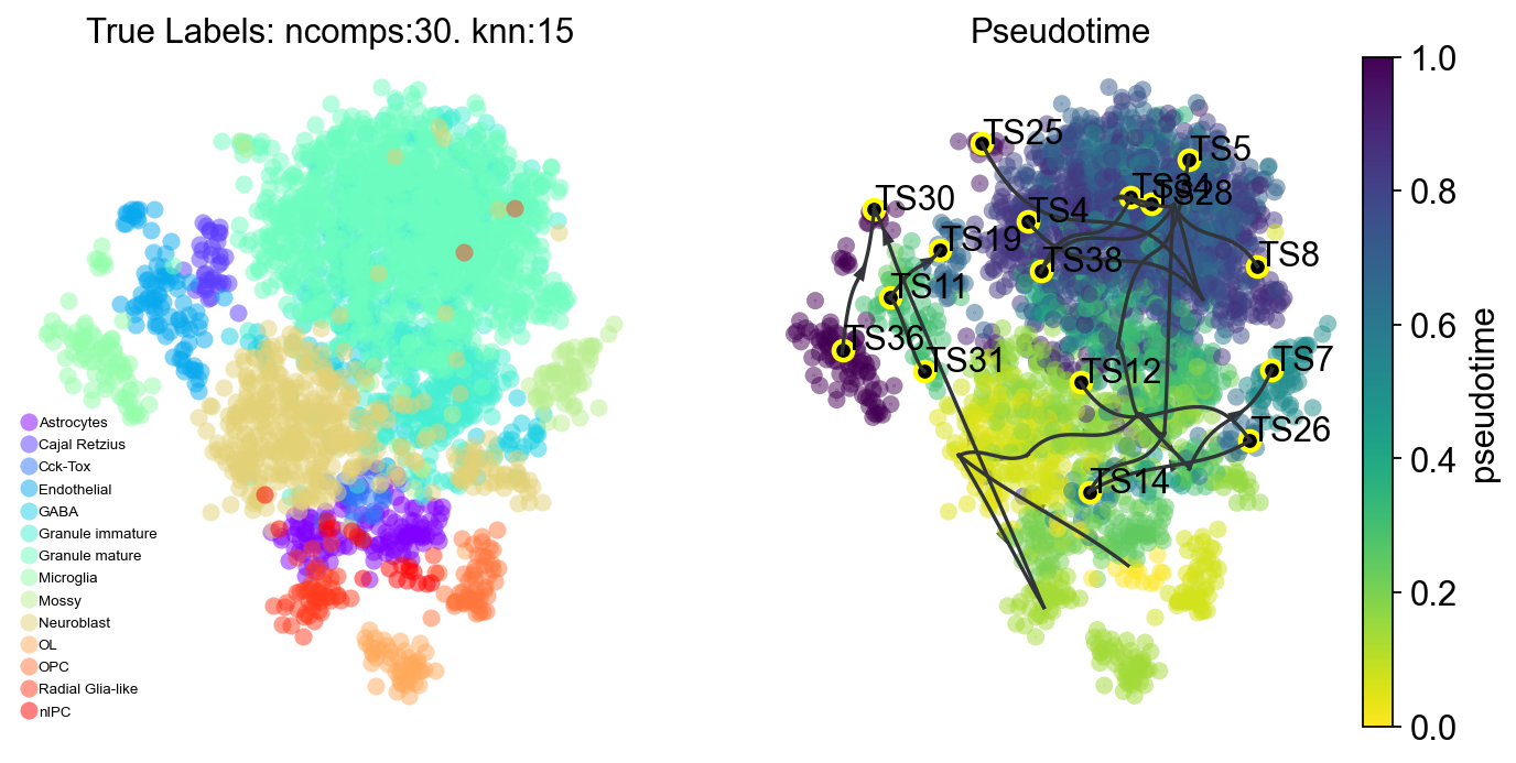
StaVIA 图结构和伪时间#
fig, ax, ax1 = VIA.core.plot_piechart_viagraph(
    via_object=v0,
    dpi=80,
    ax_text=False,
    show_legend=False,
)
fig.set_size_inches(8, 4)
plt.show()
tune edges False
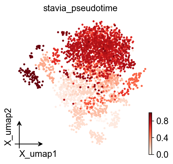
ov.pl.embedding(
    adata,
    basis="X_umap",
    color=[stavia.pseudotime_key],
    frameon="small",
    cmap="Reds",
)
StaVIA 轨迹投影#
fig, ax, ax1 = VIA.core.plot_trajectory_curves(
    via_object=v0,
    embedding=stavia_embedding,
    dpi=80,
    draw_all_curves=False,
)
fig.set_size_inches(10, 5)
plt.show()
2026-05-23 03:41:25.502983	Super cluster 4 is a super terminal with sub_terminal cluster 34
2026-05-23 03:41:25.503113	Super cluster 5 is a super terminal with sub_terminal cluster 4
2026-05-23 03:41:25.503133	Super cluster 7 is a super terminal with sub_terminal cluster 5
2026-05-23 03:41:25.503150	Super cluster 8 is a super terminal with sub_terminal cluster 36
2026-05-23 03:41:25.503171	Super cluster 11 is a super terminal with sub_terminal cluster 7
2026-05-23 03:41:25.503187	Super cluster 12 is a super terminal with sub_terminal cluster 8
2026-05-23 03:41:25.503207	Super cluster 14 is a super terminal with sub_terminal cluster 38
2026-05-23 03:41:25.503226	Super cluster 19 is a super terminal with sub_terminal cluster 11
2026-05-23 03:41:25.503245	Super cluster 25 is a super terminal with sub_terminal cluster 12
2026-05-23 03:41:25.503260	Super cluster 26 is a super terminal with sub_terminal cluster 14
2026-05-23 03:41:25.503280	Super cluster 28 is a super terminal with sub_terminal cluster 19
2026-05-23 03:41:25.503297	Super cluster 30 is a super terminal with sub_terminal cluster 25
2026-05-23 03:41:25.503316	Super cluster 31 is a super terminal with sub_terminal cluster 26
2026-05-23 03:41:25.503337	Super cluster 34 is a super terminal with sub_terminal cluster 28
2026-05-23 03:41:25.503354	Super cluster 36 is a super terminal with sub_terminal cluster 30
2026-05-23 03:41:25.503369	Super cluster 38 is a super terminal with sub_terminal cluster 31
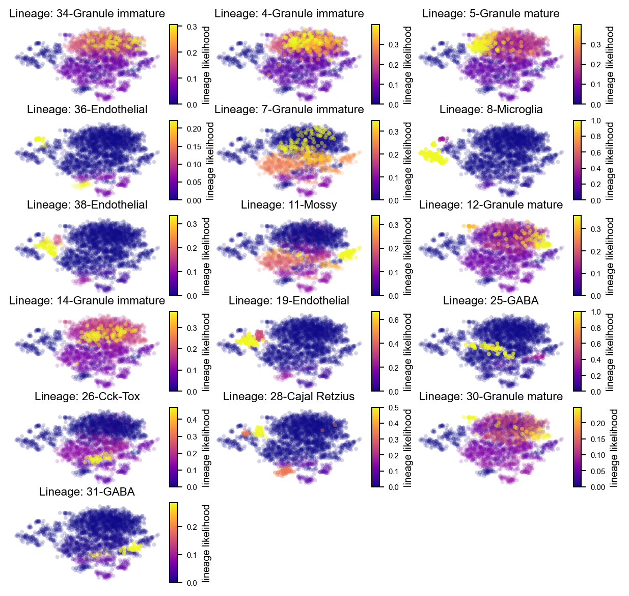
StaVIA 谱系概率#
参考 t_via.ipynb 中的 probabilistic pathways 小节,先展示所有终末谱系概率,再选择前两个终末谱系单独查看。
fig, axs = VIA.core.plot_sc_lineage_probability(
    via_object=v0,
    embedding=stavia_embedding,
    dpi=90,
)
fig.set_size_inches(8, 8)
plt.show()
2026-05-23 03:41:25.869588	Marker_lineages: [34, 4, 5, 36, 7, 8, 38, 11, 12, 14, 19, 25, 26, 28, 30, 31]
2026-05-23 03:41:25.870170	The number of components in the original full graph is 1
2026-05-23 03:41:25.870182	For downstream visualization purposes we are also constructing a low knn-graph
2026-05-23 03:41:29.145889	Check sc pb 1.0
f getting majority comp
2026-05-23 03:41:29.172291	Cluster path on clustergraph starting from Root Cluster 33 to Terminal Cluster 34: [33, 23, 27, 9, 1, 3, 24, 18, 37, 6, 34]
2026-05-23 03:41:29.172308	Cluster path on clustergraph starting from Root Cluster 33 to Terminal Cluster 4: [33, 23, 27, 9, 1, 3, 24, 18, 37, 6, 34, 4]
2026-05-23 03:41:29.172315	Cluster path on clustergraph starting from Root Cluster 33 to Terminal Cluster 5: [33, 23, 27, 9, 1, 3, 24, 18, 37, 6, 5]
2026-05-23 03:41:29.172321	Cluster path on clustergraph starting from Root Cluster 33 to Terminal Cluster 36: [33, 23, 21, 40, 36]
2026-05-23 03:41:29.172327	Cluster path on clustergraph starting from Root Cluster 33 to Terminal Cluster 7: [33, 23, 27, 9, 29, 7]
2026-05-23 03:41:29.172333	Cluster path on clustergraph starting from Root Cluster 33 to Terminal Cluster 8: [33, 23, 21, 40, 36, 8]
2026-05-23 03:41:29.172338	Cluster path on clustergraph starting from Root Cluster 33 to Terminal Cluster 38: [33, 23, 21, 40, 19, 38]
2026-05-23 03:41:29.172352	Cluster path on clustergraph starting from Root Cluster 33 to Terminal Cluster 11: [33, 23, 27, 9, 29, 11]
2026-05-23 03:41:29.172358	Cluster path on clustergraph starting from Root Cluster 33 to Terminal Cluster 12: [33, 23, 27, 9, 1, 3, 24, 18, 35, 12]
2026-05-23 03:41:29.172364	Cluster path on clustergraph starting from Root Cluster 33 to Terminal Cluster 14: [33, 23, 27, 9, 1, 3, 24, 18, 35, 14]
2026-05-23 03:41:29.172369	Cluster path on clustergraph starting from Root Cluster 33 to Terminal Cluster 19: [33, 23, 21, 40, 19]
2026-05-23 03:41:29.172374	Cluster path on clustergraph starting from Root Cluster 33 to Terminal Cluster 25: [33, 23, 27, 9, 1, 3, 24, 26, 31, 25]
2026-05-23 03:41:29.172380	Cluster path on clustergraph starting from Root Cluster 33 to Terminal Cluster 26: [33, 23, 27, 9, 1, 3, 24, 26]
2026-05-23 03:41:29.172385	Cluster path on clustergraph starting from Root Cluster 33 to Terminal Cluster 28: [33, 23, 21, 40, 28]
2026-05-23 03:41:29.172390	Cluster path on clustergraph starting from Root Cluster 33 to Terminal Cluster 30: [33, 23, 27, 9, 1, 3, 24, 18, 35, 12, 30]
2026-05-23 03:41:29.172395	Cluster path on clustergraph starting from Root Cluster 33 to Terminal Cluster 31: [33, 23, 27, 9, 1, 3, 24, 26, 31]
setting vmin to 0.0
2026-05-23 03:41:29.215068	Revised Cluster level path on sc-knnGraph from Root Cluster 33 to Terminal Cluster 34 along path: [16, 16, 10, 21, 40, 18, 14, 14, 14]
setting vmin to 0.0
2026-05-23 03:41:29.221367	Revised Cluster level path on sc-knnGraph from Root Cluster 33 to Terminal Cluster 4 along path: [16, 16, 10, 21, 40, 18, 14, 4]
setting vmin to 0.0
2026-05-23 03:41:29.227956	Revised Cluster level path on sc-knnGraph from Root Cluster 33 to Terminal Cluster 5 along path: [16, 16, 10, 21, 40, 18, 7, 5, 5]
setting vmin to 0.0
2026-05-23 03:41:29.234514	Revised Cluster level path on sc-knnGraph from Root Cluster 33 to Terminal Cluster 36 along path: [16, 16, 10, 21, 40, 36, 36]
setting vmin to 0.0
2026-05-23 03:41:29.241830	Revised Cluster level path on sc-knnGraph from Root Cluster 33 to Terminal Cluster 7 along path: [16, 16, 10, 21, 40, 18, 7, 7, 7, 7]
setting vmin to 0.0
2026-05-23 03:41:29.248418	Revised Cluster level path on sc-knnGraph from Root Cluster 33 to Terminal Cluster 8 along path: [16, 16, 10, 21, 40, 36, 8, 8, 8]
setting vmin to 0.0
2026-05-23 03:41:29.254714	Revised Cluster level path on sc-knnGraph from Root Cluster 33 to Terminal Cluster 38 along path: [16, 16, 10, 21, 40, 19, 38, 38]
setting vmin to 0.0
2026-05-23 03:41:29.261759	Revised Cluster level path on sc-knnGraph from Root Cluster 33 to Terminal Cluster 11 along path: [16, 16, 10, 21, 40, 18, 7, 11, 11, 11, 11]
setting vmin to 0.0
2026-05-23 03:41:29.268477	Revised Cluster level path on sc-knnGraph from Root Cluster 33 to Terminal Cluster 12 along path: [16, 16, 10, 21, 40, 18, 12, 12, 12]
setting vmin to 0.0
2026-05-23 03:41:29.275213	Revised Cluster level path on sc-knnGraph from Root Cluster 33 to Terminal Cluster 14 along path: [16, 16, 10, 21, 40, 18, 12, 12]
setting vmin to 0.0
2026-05-23 03:41:29.282351	Revised Cluster level path on sc-knnGraph from Root Cluster 33 to Terminal Cluster 19 along path: [16, 16, 10, 21, 40, 19, 19, 19]
setting vmin to 0.0
2026-05-23 03:41:29.288796	Revised Cluster level path on sc-knnGraph from Root Cluster 33 to Terminal Cluster 25 along path: [16, 16, 16, 16, 21, 23, 33, 27, 17, 17, 17]
setting vmin to 0.0
2026-05-23 03:41:29.294889	Revised Cluster level path on sc-knnGraph from Root Cluster 33 to Terminal Cluster 26 along path: [16, 16, 16, 16, 21, 23, 2, 2, 2]
setting vmin to 0.0
2026-05-23 03:41:29.301869	Revised Cluster level path on sc-knnGraph from Root Cluster 33 to Terminal Cluster 28 along path: [16, 16, 10, 21, 40, 28, 28, 28]
setting vmin to 0.0
2026-05-23 03:41:29.308393	Revised Cluster level path on sc-knnGraph from Root Cluster 33 to Terminal Cluster 30 along path: [16, 16, 10, 21, 40, 18, 5, 5]
setting vmin to 0.0
2026-05-23 03:41:29.314790	Revised Cluster level path on sc-knnGraph from Root Cluster 33 to Terminal Cluster 31 along path: [16, 16, 16, 16, 21, 23, 2, 31, 31, 31]
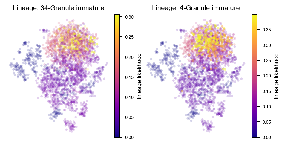
marker_lineages = list(v0.terminal_clusters)[:2]

fig, axs = VIA.core.plot_sc_lineage_probability(
    via_object=v0,
    embedding=stavia_embedding,
    marker_lineages=marker_lineages,
    dpi=90,
)
fig.set_size_inches(6, 3)
plt.show()
2026-05-23 03:41:29.802128	Marker_lineages: [34, 4]
2026-05-23 03:41:29.802668	The number of components in the original full graph is 1
2026-05-23 03:41:29.802678	For downstream visualization purposes we are also constructing a low knn-graph
2026-05-23 03:41:33.039376	Check sc pb 1.0
f getting majority comp
2026-05-23 03:41:33.062977	Cluster path on clustergraph starting from Root Cluster 33 to Terminal Cluster 34: [33, 23, 27, 9, 1, 3, 24, 18, 37, 6, 34]
2026-05-23 03:41:33.062994	Cluster path on clustergraph starting from Root Cluster 33 to Terminal Cluster 4: [33, 23, 27, 9, 1, 3, 24, 18, 37, 6, 34, 4]
setting vmin to 0.0
2026-05-23 03:41:33.074485	Revised Cluster level path on sc-knnGraph from Root Cluster 33 to Terminal Cluster 34 along path: [16, 16, 10, 21, 40, 18, 14, 14, 14]
setting vmin to 0.0
2026-05-23 03:41:33.080987	Revised Cluster level path on sc-knnGraph from Root Cluster 33 to Terminal Cluster 4 along path: [16, 16, 10, 21, 40, 18, 14, 4]
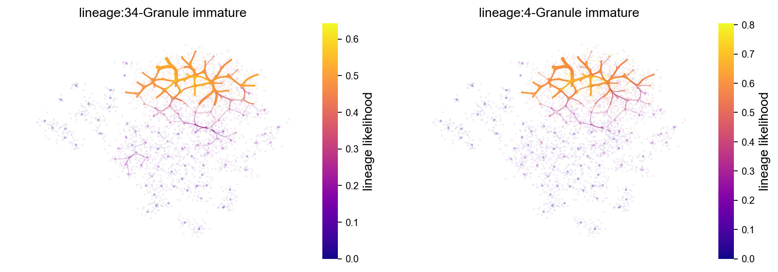
StaVIA 谱系路径 atlas 图#
lineage_pathway = list(v0.terminal_clusters)[:2]

fig, axs = VIA.core.plot_atlas_view(
    via_object=v0,
    dpi=80,
    lineage_pathway=lineage_pathway,
    fontsize_title=12,
    fontsize_labels=12,
)
fig.set_size_inches(12, 4)
plt.show()
location of 34 is at [0] and 0
setting vmin to 0.0
location of 4 is at [1] and 1
setting vmin to 0.0
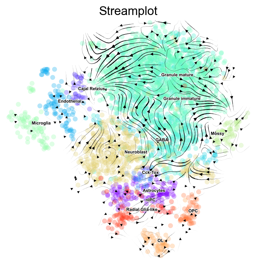
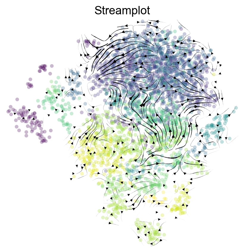
StaVIA 流线图#
参考 t_via.ipynb 中的 stream plot 示例,分别展示按注释着色的流线图和按伪时间着色的流线图。
fig, ax = VIA.core.via_streamplot(
    via_object=v0,
    embedding=stavia_embedding,
    dpi=100,
    density_stream=2.5,
    linewidth=0.8,
    density_grid=0.8,
    scatter_size=30,
    scatter_alpha=0.3,
)
fig.set_size_inches(5, 5)
plt.show()
fig, ax = VIA.core.via_streamplot(
    via_object=v0,
    embedding=stavia_embedding,
    dpi=100,
    density_grid=1.0,
    density_stream=2.5,
    scatter_size=18,
    scatter_alpha=0.28,
    linewidth=0.8,
    color_scheme="time",
    min_mass=1,
    cutoff_perc=5,
    marker_edgewidth=0.1,
    smooth_transition=1,
    smooth_grid=0.5,
)
fig.set_size_inches(5, 5)
plt.show()
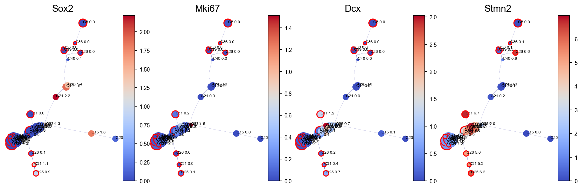
可视化基因/特征图#
使用拟合后的 VIA 图对选定基因进行 MAGIC-like 平滑,再展示 cluster 水平的基因变化。
stavia_marker_genes = [
    gene
    for gene in ["Sox2", "Mki67", "Dcx", "Neurod1", "Stmn2", "Prox1"]
    if gene in adata.raw.var_names
]

df_gene = adata.raw[:, stavia_marker_genes].to_adata().to_df()
df_magic = v0.do_impute(
    df_gene,
    magic_steps=3,
    gene_list=stavia_marker_genes,
)
shape of transition matrix raised to power 3 (2930, 2930)
fig, axs = VIA.core.plot_viagraph(
    via_object=v0,
    type_data="gene",
    df_genes=df_magic.copy(),
    gene_list=stavia_marker_genes[:4],
    arrow_head=0.1,
)
fig.set_size_inches(12, 4)
plt.show()
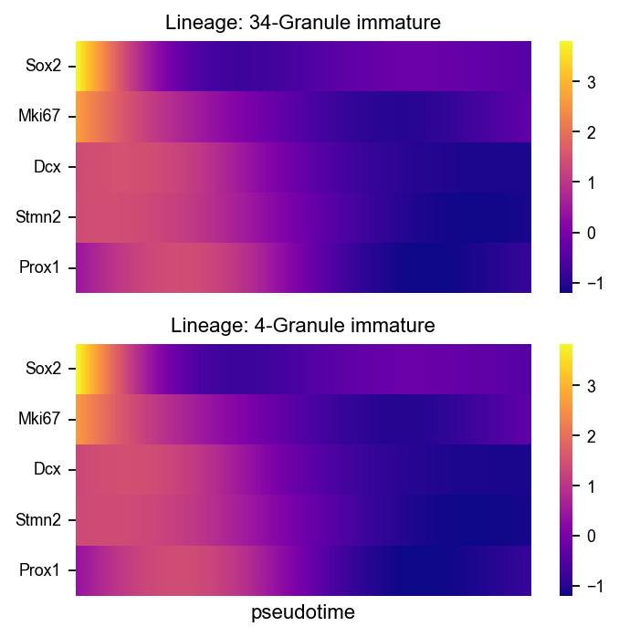
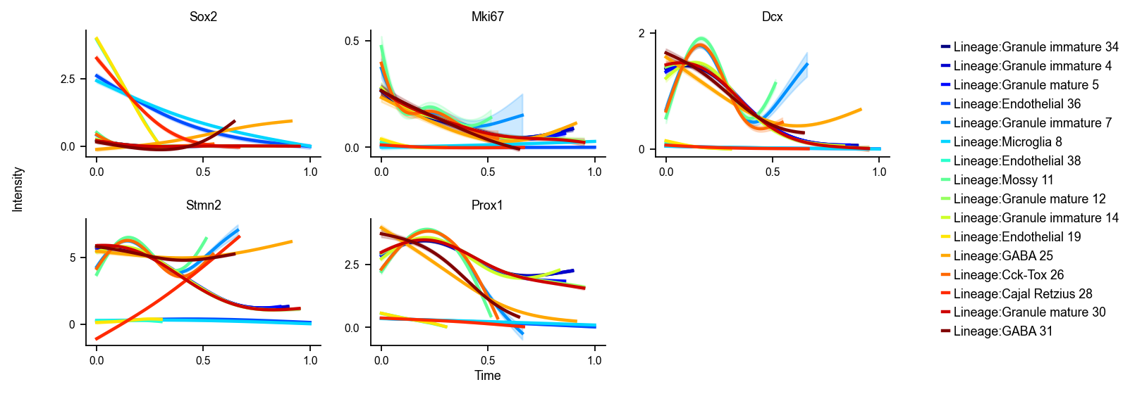
StaVIA 谱系基因动态#
VIA 会沿检测到的终末谱系估计伪时间上的基因动态。
fig, axs = VIA.core.get_gene_expression(
    via_object=v0,
    gene_exp=df_magic[stavia_marker_genes],
    marker_genes=stavia_marker_genes,
    dpi=80,
    figsize=(10, 4),
    ncols=3,
    legend_loc="right",
)
plt.show()
Area under curve Sox2 for branch Granule immature is 0.01742602766299818
Area under curve Sox2 for branch Granule immature is 0.0175467416298079
Area under curve Sox2 for branch Granule mature is 0.01811803163437256
Area under curve Sox2 for branch Endothelial is 0.8584266954933628
Area under curve Sox2 for branch Granule immature is 0.018846090759457982
Area under curve Sox2 for branch Microglia is 0.9749461155541378
Area under curve Sox2 for branch Endothelial is 0.574162475007691
Area under curve Sox2 for branch Mossy is 0.02147413469772736
Area under curve Sox2 for branch Granule mature is 0.01802916926037789
Area under curve Sox2 for branch Granule immature is 0.018542996303335724
Area under curve Sox2 for branch Endothelial is 0.5747433267188964
Area under curve Sox2 for branch GABA is 0.33469202085015787
Area under curve Sox2 for branch Cck-Tox is 0.024012462787964064
Area under curve Sox2 for branch Cajal Retzius is 0.6424109202817495
Area under curve Sox2 for branch Granule mature is 0.018167166323069667
Area under curve Sox2 for branch GABA is 0.06097160635457299
Area under curve Mki67 for branch Granule immature is 0.09331821451874674
Area under curve Mki67 for branch Granule immature is 0.0953108628939297
Area under curve Mki67 for branch Granule mature is 0.09136530637217873
Area under curve Mki67 for branch Endothelial is 0.0011614819476727617
Area under curve Mki67 for branch Granule immature is 0.10189161879935847
Area under curve Mki67 for branch Microglia is 0.012658691290116458
Area under curve Mki67 for branch Endothelial is 0.0018278916798260296
Area under curve Mki67 for branch Mossy is 0.08775252848894795
Area under curve Mki67 for branch Granule mature is 0.09418439576323992
Area under curve Mki67 for branch Granule immature is 0.09037124887575845
Area under curve Mki67 for branch Endothelial is 0.002525148277880088
Area under curve Mki67 for branch GABA is 0.08204476875032032
Area under curve Mki67 for branch Cck-Tox is 0.07914979716400126
Area under curve Mki67 for branch Cajal Retzius is 0.0008077918360658437
Area under curve Mki67 for branch Granule mature is 0.09316653870291516
Area under curve Mki67 for branch GABA is 0.07414913196752643
Area under curve Dcx for branch Granule immature is 0.5914164221481015
Area under curve Dcx for branch Granule immature is 0.5971225495031912
Area under curve Dcx for branch Granule mature is 0.5993491247799094
Area under curve Dcx for branch Endothelial is 0.02141181521365349
Area under curve Dcx for branch Granule immature is 0.7180517431330387
Area under curve Dcx for branch Microglia is 0.02131113895284662
Area under curve Dcx for branch Endothelial is 0.013316232324289301
Area under curve Dcx for branch Mossy is 0.5928319184002112
Area under curve Dcx for branch Granule mature is 0.5892080843229042
Area under curve Dcx for branch Granule immature is 0.5858709777876406
Area under curve Dcx for branch Endothelial is 0.014844139550161412
Area under curve Dcx for branch GABA is 0.6815596124096264
Area under curve Dcx for branch Cck-Tox is 0.5437276441010759
Area under curve Dcx for branch Cajal Retzius is 0.01606743050384075
Area under curve Dcx for branch Granule mature is 0.5901582189193307
Area under curve Dcx for branch GABA is 0.5780603393649969
Area under curve Stmn2 for branch Granule immature is 2.968069546302115
Area under curve Stmn2 for branch Granule immature is 2.9908637410289414
Area under curve Stmn2 for branch Granule mature is 2.966475495536181
Area under curve Stmn2 for branch Endothelial is 0.30788619483375845
Area under curve Stmn2 for branch Granule immature is 3.4790288048234066
Area under curve Stmn2 for branch Microglia is 0.22978883840495418
Area under curve Stmn2 for branch Endothelial is 0.07612164331615864
Area under curve Stmn2 for branch Mossy is 2.6875925481758154
Area under curve Stmn2 for branch Granule mature is 2.997020905247549
Area under curve Stmn2 for branch Granule immature is 2.906218968903863
Area under curve Stmn2 for branch Endothelial is 0.08285643039178402
Area under curve Stmn2 for branch GABA is 4.8422931924721055
Area under curve Stmn2 for branch Cck-Tox is 2.6594940650005334
Area under curve Stmn2 for branch Cajal Retzius is 1.6246413925833685
Area under curve Stmn2 for branch Granule mature is 3.002783220091677
Area under curve Stmn2 for branch GABA is 3.322215285490052
Area under curve Prox1 for branch Granule immature is 2.4134114927671986
Area under curve Prox1 for branch Granule immature is 2.4126578202359936
Area under curve Prox1 for branch Granule mature is 2.2835473248271208
Area under curve Prox1 for branch Endothelial is 0.20380427195086076
Area under curve Prox1 for branch Granule immature is 1.6100151501895155
Area under curve Prox1 for branch Microglia is 0.2312176581925458
Area under curve Prox1 for branch Endothelial is 0.09082244514466213
Area under curve Prox1 for branch Mossy is 1.5068780656071614
Area under curve Prox1 for branch Granule mature is 2.457800584727098
Area under curve Prox1 for branch Granule immature is 2.2562023054180784
Area under curve Prox1 for branch Endothelial is 0.09191063724807158
Area under curve Prox1 for branch GABA is 1.508677947593942
Area under curve Prox1 for branch Cck-Tox is 1.572493629155324
Area under curve Prox1 for branch Cajal Retzius is 0.15190777822870574
Area under curve Prox1 for branch Granule mature is 2.4443331178685828
Area under curve Prox1 for branch GABA is 1.4731009483632156
marker_lineages = list(v0.terminal_clusters)[:2]

fig, axs = VIA.core.plot_gene_trend_heatmaps(
    via_object=v0,
    df_gene_exp=df_magic[stavia_marker_genes],
    cmap="plasma",
    marker_lineages=marker_lineages,
)
fig.set_size_inches(5, max(3, 2.5 * len(marker_lineages)))
plt.show()
branches [34, 4]