使用 VIA 进行轨迹推断#
VIA(Velocity and Topology Inference Algorithm)是一种单细胞轨迹推断方法,可以同时完成轨迹拓扑构建、伪时间估计、终末状态自动识别,以及沿谱系的基因动态可视化。本教程基于 VIA 作者提供的示例数据和分析流程,并在 OmicVerse 中提供更贴近 AnnData 使用习惯的包装接口。
如果在研究中使用 VIA,请引用:
Generalized and scalable trajectory inference in single-cell omics data with VIA
代码仓库:ShobiStassen/VIA
Colab 可复现教程:https://colab.research.google.com/drive/1A2X23z_RLJaYLbXaiCbZa-fjNbuGACrD?usp=sharing
%matplotlib inline

from pathlib import Path
import warnings

import scanpy as sc
import matplotlib.pyplot as plt
import omicverse as ov

warnings.filterwarnings("ignore", category=FutureWarning)

ov.plot_set(font_path='Arial')
Path("figures").mkdir(exist_ok=True)

%load_ext autoreload
%autoreload 2
🔬 Starting plot initialization...
Using already downloaded Arial font from: /var/folders/rv/3jnfbs0d6r7d0c5bfj7ft5k00000gn/T/omicverse_arial.ttf
Registered as: Arial
🧬 Detecting GPU devices…
✅ Apple Silicon MPS detected
    • [MPS] Apple Silicon GPU - Metal Performance Shaders available

   ____            _     _    __
  / __ \____ ___  (_)___| |  / /__  _____________
 / / / / __ `__ \/ / ___/ | / / _ \/ ___/ ___/ _ \
/ /_/ / / / / / / / /__ | |/ /  __/ /  (__  )  __/
\____/_/ /_/ /_/_/\___/ |___/\___/_/  /____/\___/

🔖 Version: 2.2.1rc1   📚 Tutorials: https://omicverse.readthedocs.io/
✅ plot_set complete.
数据加载与预处理#
本教程使用 VIA 作者提供的 scRNA_hematopoiesis 造血发育数据集。该数据已经完成标准化和对数转换,但尚未进行 scaling。载入数据后,我们先计算 PCA,后续 VIA 会使用 adata.obsm["X_pca"] 作为细胞特征空间。
adata = ov.single.scRNA_hematopoiesis()
sc.tl.pca(adata, svd_solver='arpack', n_comps=200)
adata
Cell type B_a1 has  27 cells
Cell type GMP has  28 cells
Cell type MEP has  339 cells
Cell type ERY1 has  773 cells
Cell type PRE_B3 has  2 cells
Cell type B_a4 has  8 cells
Cell type PRE_B2 has  515 cells
Cell type ERY4 has  53 cells
Cell type GRAN1 has  3 cells
Cell type BASO1 has  2 cells
Cell type EOS2 has  3 cells
Cell type HSC2 has  10 cells
Cell type mDC (cDC) has  96 cells
Cell type ERY3 has  104 cells
Cell type MEGA1 has  12 cells
Cell type B_a2 has  1 cells
Cell type MONO2 has  35 cells
Cell type pDC has  204 cells
Cell type TCEL7 has  1 cells
Cell type MONO1 has  186 cells
Cell type HSC1 has  2365 cells
Cell type ERY2 has  40 cells
Cell type CMP has  968 cells
Cell type Nka3 has  5 cells
AnnData object with n_obs × n_vars = 5780 × 14651
    obs: 'clusters', 'palantir_pseudotime', 'palantir_diff_potential', 'label'
    uns: 'cluster_colors', 'ct_colors', 'palantir_branch_probs_cell_types', 'pca'
    obsm: 'tsne', 'MAGIC_imputed_data', 'palantir_branch_probs', 'X_pca'
    varm: 'PCs'
构建并运行 VIA 模型#
运行 VIA 时需要指定用于轨迹推断的细胞特征矩阵,例如 X_pca、X_scVI 或 X_glue。这里使用 X_pca,并通过 adata_ncomps=80 指定前 80 个主成分。
还需要指定用于着色和图结构汇总的细胞注释列 clusters。本教程使用 adata.obs["label"]。如果不提供 root_user,VIA 会尝试自动选择根细胞;这里为了复现作者示例,显式指定根细胞索引。二维展示坐标由 basis 指定,本数据集中可使用 adata.obsm["tsne"]。
更多参数说明可参考 VIA 文档:https://pyvia.readthedocs.io/en/latest/Parameters and Attributes.html
v0 = ov.single.pyVIA(
    adata=adata,
    adata_key='X_pca',
    adata_ncomps=80,
    basis='tsne',
    clusters='label',
    knn=30,
    random_seed=4,
    root_user=[4823],
)

v0.run()

via_marker_lineages = list(v0.model.terminal_clusters)[:2]
via_heatmap_lineages = via_marker_lineages[:1]
print(f"Selected terminal lineages: {via_marker_lineages}")
2026-05-23 00:35:19.967832	Running VIA over input data of 5780 (samples) x 80 (features)
2026-05-23 00:35:19.967913	Knngraph has 30 neighbors
2026-05-23 00:35:22.271938	Finished global pruning of 30-knn graph used for clustering at level of 0.15. Kept 46.3 % of edges.
2026-05-23 00:35:22.285443	Number of connected components used for clustergraph  is 1
2026-05-23 00:35:22.421842	Commencing community detection
2026-05-23 00:35:22.788173	Finished community detection. Found 207 clusters.
2026-05-23 00:35:22.789278	Merging 189 very small clusters (<10)
2026-05-23 00:35:22.790632	Finished detecting communities. Found 18 communities
2026-05-23 00:35:22.790796	Making cluster graph. Global cluster graph pruning level: 0.15
2026-05-23 00:35:22.799106	Graph has 1 connected components before pruning
2026-05-23 00:35:22.799869	Graph has 2 connected components after pruning
2026-05-23 00:35:22.800252	Graph has 1 connected components after reconnecting
2026-05-23 00:35:22.800414	0.0% links trimmed from local pruning relative to start
2026-05-23 00:35:22.800424	62.6% links trimmed from global pruning relative to start
initial links 198 and final_links_n 198
2026-05-23 00:35:22.801501	component number 0 out of  [0]
2026-05-23 00:35:22.821427	The root index, 4823 provided by the user belongs to cluster number 2 and corresponds to cell type HSC1
2026-05-23 00:35:22.822267	Computing lazy-teleporting expected hitting times
2026-05-23 00:35:27.012630	Ended all multiprocesses, will retrieve and reshape
2026-05-23 00:35:27.026042	start computing walks with rw2 method
memory for rw2 hittings times  2. Using rw2 based pt
2026-05-23 00:35:30.092010	Identifying terminal clusters corresponding to unique lineages...
2026-05-23 00:35:30.092025	Closeness:[3, 5, 7, 9, 12, 14]
2026-05-23 00:35:30.092031	Betweenness:[1, 2, 3, 4, 7, 9, 10, 12, 14, 15, 16]
2026-05-23 00:35:30.092036	Out Degree:[3, 4, 5, 9, 10, 12, 14, 15, 16]
2026-05-23 00:35:30.092096	Cluster 5 had 3 or more neighboring terminal states [7, 9, 16] and so we removed cluster 7
2026-05-23 00:35:30.092111	We removed cluster 10 from the shortlist of terminal states
2026-05-23 00:35:30.092160	Terminal clusters corresponding to unique lineages in this component are [3, 4, 5, 9, 12, 14, 15, 16]
2026-05-23 00:35:30.092168	Calculating lineage probability at memory 5
2026-05-23 00:35:31.766889	Cluster or terminal cell fate 3 is reached 19.0 times
2026-05-23 00:35:31.783154	Cluster or terminal cell fate 4 is reached 423.0 times
2026-05-23 00:35:31.798511	Cluster or terminal cell fate 5 is reached 84.0 times
2026-05-23 00:35:31.811931	Cluster or terminal cell fate 9 is reached 84.0 times
2026-05-23 00:35:31.823678	Cluster or terminal cell fate 12 is reached 416.0 times
2026-05-23 00:35:31.834526	Cluster or terminal cell fate 14 is reached 559.0 times
2026-05-23 00:35:31.845602	Cluster or terminal cell fate 15 is reached 543.0 times
2026-05-23 00:35:31.859101	Cluster or terminal cell fate 16 is reached 54.0 times
2026-05-23 00:35:31.861442	There are (8) terminal clusters corresponding to unique lineages {3: 'PRE_B2', 4: 'CMP', 5: 'ERY1', 9: 'ERY1', 12: 'MONO1', 14: 'pDC', 15: 'pDC', 16: 'ERY1'}
2026-05-23 00:35:31.861455	Begin projection of pseudotime and lineage likelihood
2026-05-23 00:35:32.785927	Cluster graph layout based on forward biasing
2026-05-23 00:35:32.786490	Starting make edgebundle viagraph...
2026-05-23 00:35:34.701253	Make via clustergraph edgebundle
2026-05-23 00:35:34.849123	Hammer dims: Nodes shape: (18, 2) Edges shape: (74, 3)
2026-05-23 00:35:34.849439	Graph has 1 connected components before pruning
2026-05-23 00:35:34.849976	Graph has 6 connected components after pruning
2026-05-23 00:35:34.851021	Graph has 1 connected components after reconnecting
2026-05-23 00:35:34.851163	52.7% links trimmed from local pruning relative to start
2026-05-23 00:35:34.851174	63.5% links trimmed from global pruning relative to start
initial links 74 and final_links_n 35
2026-05-23 00:35:34.851983	Start making edgebundle milestone with 150 milestones...This can be recomputed with make_edgebundle_milestone()
2026-05-23 00:35:34.851995	Start finding milestones
2026-05-23 00:35:36.160995	End milestones with 150
2026-05-23 00:35:36.161140	Will use via-pseudotime for edges, otherwise consider providing a list of numeric labels (single cell level) or via_object
2026-05-23 00:35:36.180081	Recompute weights
2026-05-23 00:35:36.193787	pruning milestone graph based on recomputed weights
2026-05-23 00:35:36.195124	Graph has 1 connected components before pruning
2026-05-23 00:35:36.195705	Graph has 1 connected components after pruning
2026-05-23 00:35:36.195829	Graph has 1 connected components after reconnecting
2026-05-23 00:35:36.196301	68.6% links trimmed from global pruning relative to start
2026-05-23 00:35:36.196319	regenerate igraph on pruned edges
2026-05-23 00:35:36.200082	Setting numeric label as single cell pseudotime for coloring edges
2026-05-23 00:35:36.210034	Making smooth edges
REMEMBER TO RE-INCLUDE the PLT.SHOW HERE - COMMENTING IT OUT FOR NOW
2026-05-23 00:35:36.530599	Time elapsed 15.5 seconds
Selected terminal lineages: [3, 4]
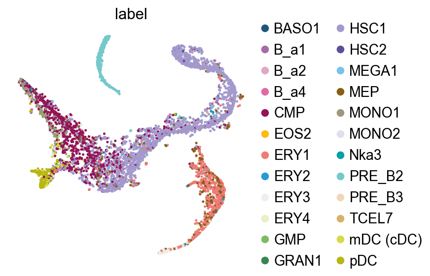
基础可视化#
在后续轨迹图之前,先查看细胞注释在 tSNE 空间中的分布。
fig, ax = plt.subplots(1,1,figsize=(4,4))
ov.pl.embedding(
    adata,
    basis="tsne",
    color=['label'],
    frameon=False,
    ncols=1,
    wspace=0.5,
    show=False,
    ax=ax
)
fig.savefig('figures/via_fig1.png',dpi=300,bbox_inches = 'tight')
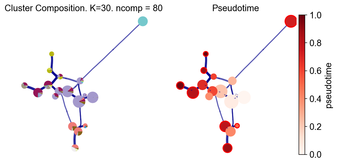
VIA 图结构#
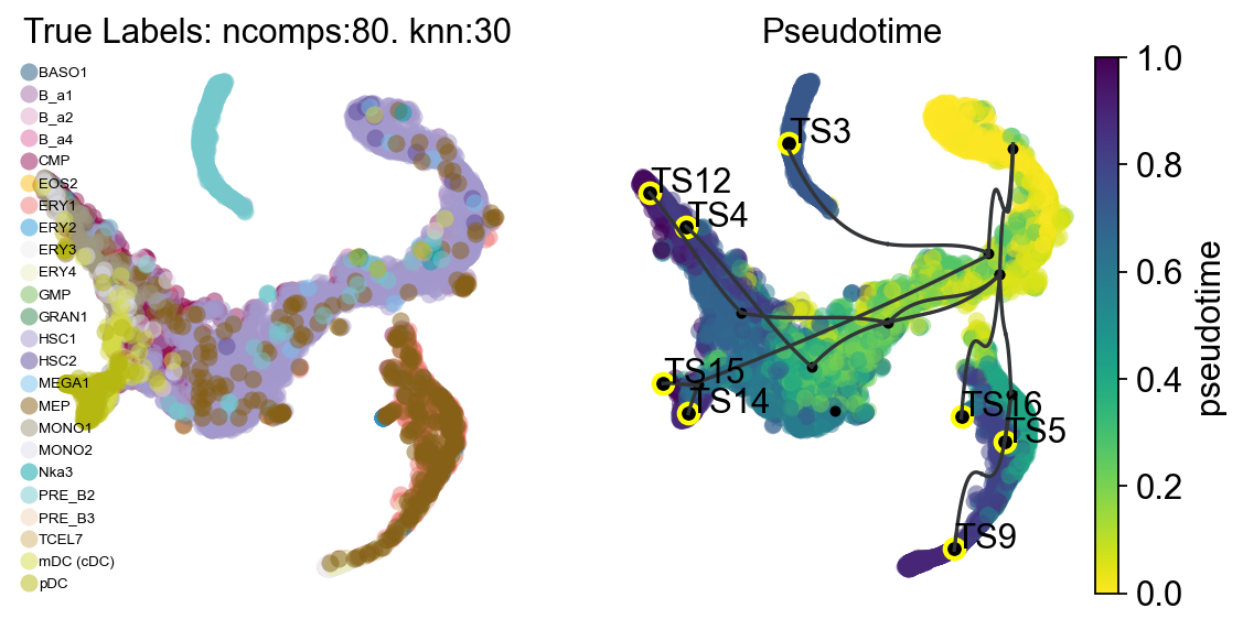
VIA 提供多种轨迹可视化方式。这里先展示 cluster graph 层面的轨迹抽象:左图显示每个 VIA cluster 中真实注释标签的组成,右图显示 VIA 推断的伪时间。这个视图适合快速检查整体拓扑、根位置和终末分支是否符合预期。
fig, ax, ax1 = v0.plot_piechart_graph(
    clusters='label',
    cmap='Reds',
    dpi=80,
    show_legend=False,
    ax_text=False,
    fontsize=4
)
fig.savefig('figures/via_fig2.png',dpi=300,bbox_inches = 'tight')
#you can use `v0.model.single_cell_pt_markov` to extract the pseudotime
v0.get_pseudotime(v0.adata)
v0.adata
...the pseudotime of VIA added to AnnData obs named `pt_via`
AnnData object with n_obs × n_vars = 5780 × 14651
    obs: 'clusters', 'palantir_pseudotime', 'palantir_diff_potential', 'label', 'pt_via'
    uns: 'cluster_colors', 'ct_colors', 'palantir_branch_probs_cell_types', 'pca', 'REFERENCE_MANU', 'label_colors_rgba', 'label_colors'
    obsm: 'tsne', 'MAGIC_imputed_data', 'palantir_branch_probs', 'X_pca'
    varm: 'PCs'
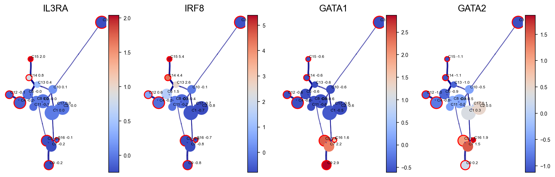
基因 / 特征图可视化#
VIA 可以沿推断得到的图结构展示基因表达变化。这里使用 VIA 内部构建的 HNSW small-world graph 加速基因表达平滑,思想上类似 MAGIC 插补。随后将选定 marker 基因投影到 VIA cluster graph 上,观察不同造血程序在轨迹中的空间分布。
gene_list_magic = ['IL3RA', 'IRF8', 'GATA1', 'GATA2', 'ITGA2B', 'MPO', 'CD79B', 'SPI1', 'CD34', 'CSF1R', 'ITGAX']
fig,axs=v0.plot_clustergraph(gene_list=gene_list_magic[:4],figsize=(12,4),)
fig.savefig('figures/via_fig2_1.png',dpi=300,bbox_inches = 'tight')
shape of transition matrix raised to power 3 (5780, 5780)
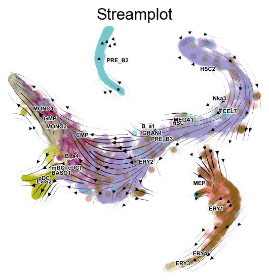
轨迹投影#
下面把 VIA 推断得到的轨迹结构投影到二维 embedding(例如 UMAP、PHATE 或 tSNE)上。这个部分包含三类视图:
将高层级 cluster graph 抽象叠加到 embedding 上;
在 embedding 上绘制更细粒度的细胞方向性向量场;
绘制高边分辨率的有向图或流线图。
fig,ax1,ax2=v0.plot_trajectory_gams(basis='tsne',clusters='label',draw_all_curves=False)
fig.savefig('figures/via_fig3.png',dpi=300,bbox_inches = 'tight')
2026-05-23 00:35:43.199713	Super cluster 3 is a super terminal with sub_terminal cluster 3
2026-05-23 00:35:43.202076	Super cluster 4 is a super terminal with sub_terminal cluster 4
2026-05-23 00:35:43.202106	Super cluster 5 is a super terminal with sub_terminal cluster 5
2026-05-23 00:35:43.202127	Super cluster 9 is a super terminal with sub_terminal cluster 9
2026-05-23 00:35:43.202144	Super cluster 12 is a super terminal with sub_terminal cluster 12
2026-05-23 00:35:43.202161	Super cluster 14 is a super terminal with sub_terminal cluster 14
2026-05-23 00:35:43.202178	Super cluster 15 is a super terminal with sub_terminal cluster 15
2026-05-23 00:35:43.202197	Super cluster 16 is a super terminal with sub_terminal cluster 16
fig,ax=v0.plot_stream(
    basis='tsne',
    clusters='label',
    density_grid=0.8,
    scatter_size=30,
    scatter_alpha=0.3,
    linewidth=0.5
)
fig.savefig('figures/via_fig4.png',dpi=300,bbox_inches = 'tight')
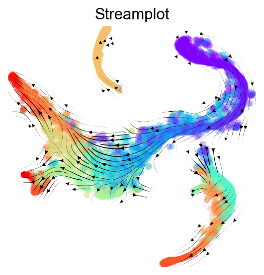
fig,ax=v0.plot_stream(
    basis='tsne',
    density_grid=0.8,
    scatter_size=30,
    color_scheme='time',
    linewidth=0.5,
    min_mass = 1,
    cutoff_perc = 5,
    scatter_alpha=0.3,
    marker_edgewidth=0.1,
    density_stream = 2,
    smooth_transition=1,
    smooth_grid=0.5
)
fig.savefig('figures/via_fig5.png',dpi=300,bbox_inches = 'tight')
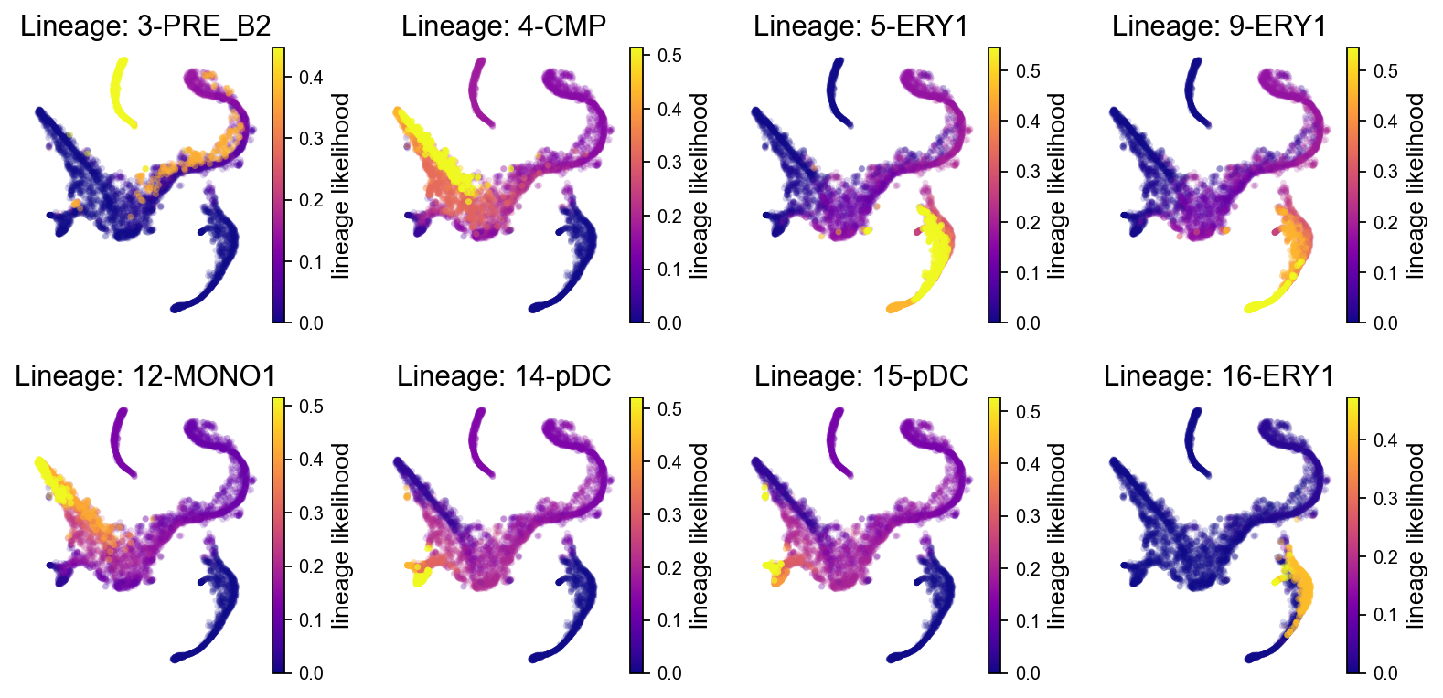
概率谱系路径#
VIA 会估计从根状态到各个终末状态的谱系概率。谱系概率越高,表示该细胞向对应终末状态分化的潜力越大。下面先展示所有终末谱系的概率分布。
fig, axs = v0.plot_lineage_probability(figsize=(10, 5),ncol=4)
fig.savefig("figures/via_fig6.png", dpi=300, bbox_inches="tight")
2026-05-23 00:35:46.098394	Marker_lineages: [3, 4, 5, 9, 12, 14, 15, 16]
2026-05-23 00:35:46.099934	The number of components in the original full graph is 1
2026-05-23 00:35:46.099951	For downstream visualization purposes we are also constructing a low knn-graph
2026-05-23 00:35:48.965546	Check sc pb 1.0
f getting majority comp
2026-05-23 00:35:49.037414	Cluster path on clustergraph starting from Root Cluster 2 to Terminal Cluster 3: [2, 1, 0, 8, 6, 13, 10, 3]
2026-05-23 00:35:49.037432	Cluster path on clustergraph starting from Root Cluster 2 to Terminal Cluster 4: [2, 1, 0, 11, 4]
2026-05-23 00:35:49.037438	Cluster path on clustergraph starting from Root Cluster 2 to Terminal Cluster 5: [2, 1, 7, 5]
2026-05-23 00:35:49.037444	Cluster path on clustergraph starting from Root Cluster 2 to Terminal Cluster 9: [2, 1, 7, 5, 9]
2026-05-23 00:35:49.037450	Cluster path on clustergraph starting from Root Cluster 2 to Terminal Cluster 12: [2, 1, 0, 8, 6, 12]
2026-05-23 00:35:49.037455	Cluster path on clustergraph starting from Root Cluster 2 to Terminal Cluster 14: [2, 1, 0, 8, 14]
2026-05-23 00:35:49.037461	Cluster path on clustergraph starting from Root Cluster 2 to Terminal Cluster 15: [2, 1, 0, 8, 6, 13, 15]
2026-05-23 00:35:49.037474	Cluster path on clustergraph starting from Root Cluster 2 to Terminal Cluster 16: [2, 1, 7, 5, 16]
setting vmin to 0.0
2026-05-23 00:35:49.060210	Revised Cluster level path on sc-knnGraph from Root Cluster 2 to Terminal Cluster 3 along path: [2, 2, 2, 1, 10, 3, 3, 3, 3, 3]
setting vmin to 0.0
2026-05-23 00:35:49.067412	Revised Cluster level path on sc-knnGraph from Root Cluster 2 to Terminal Cluster 4 along path: [2, 2, 1, 4]
setting vmin to 0.0
2026-05-23 00:35:49.075081	Revised Cluster level path on sc-knnGraph from Root Cluster 2 to Terminal Cluster 5 along path: [2, 2, 1, 16, 5, 5, 5, 5, 5]
setting vmin to 0.0
2026-05-23 00:35:49.082321	Revised Cluster level path on sc-knnGraph from Root Cluster 2 to Terminal Cluster 9 along path: [2, 2, 2, 2, 2, 1, 7, 9, 9]
setting vmin to 0.0
2026-05-23 00:35:49.089594	Revised Cluster level path on sc-knnGraph from Root Cluster 2 to Terminal Cluster 12 along path: [2, 2, 2, 1, 10, 12, 12, 12, 12, 12]
setting vmin to 0.0
2026-05-23 00:35:49.097423	Revised Cluster level path on sc-knnGraph from Root Cluster 2 to Terminal Cluster 14 along path: [2, 2, 1, 10, 13, 14, 14, 14]
setting vmin to 0.0
2026-05-23 00:35:49.104985	Revised Cluster level path on sc-knnGraph from Root Cluster 2 to Terminal Cluster 15 along path: [2, 2, 2, 10, 13, 15, 15, 15, 15]
setting vmin to 0.0
2026-05-23 00:35:49.111904	Revised Cluster level path on sc-knnGraph from Root Cluster 2 to Terminal Cluster 16 along path: [2, 2, 2, 1, 16, 16, 16, 16]
也可以只选择部分终末谱系进行可视化。这里从模型实际识别到的终末 cluster 中取前两个谱系,避免不同版本或随机种子下 cluster 编号变化导致教程失效。
fig,axs=v0.plot_lineage_probability(figsize=(8,4),marker_lineages=via_marker_lineages)
fig.savefig('figures/via_fig7.png',dpi=300,bbox_inches = 'tight')
2026-05-23 00:35:50.139048	Marker_lineages: [3, 4]
2026-05-23 00:35:50.140644	The number of components in the original full graph is 1
2026-05-23 00:35:50.140673	For downstream visualization purposes we are also constructing a low knn-graph
2026-05-23 00:35:52.890849	Check sc pb 1.0
f getting majority comp
2026-05-23 00:35:52.962141	Cluster path on clustergraph starting from Root Cluster 2 to Terminal Cluster 3: [2, 1, 0, 8, 6, 13, 10, 3]
2026-05-23 00:35:52.962158	Cluster path on clustergraph starting from Root Cluster 2 to Terminal Cluster 4: [2, 1, 0, 11, 4]
setting vmin to 0.0
2026-05-23 00:35:52.973994	Revised Cluster level path on sc-knnGraph from Root Cluster 2 to Terminal Cluster 3 along path: [2, 2, 2, 1, 10, 3, 3, 3, 3, 3]
setting vmin to 0.0
2026-05-23 00:35:52.981172	Revised Cluster level path on sc-knnGraph from Root Cluster 2 to Terminal Cluster 4 along path: [2, 2, 1, 4]

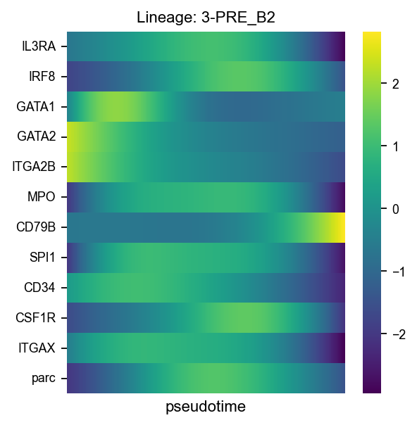
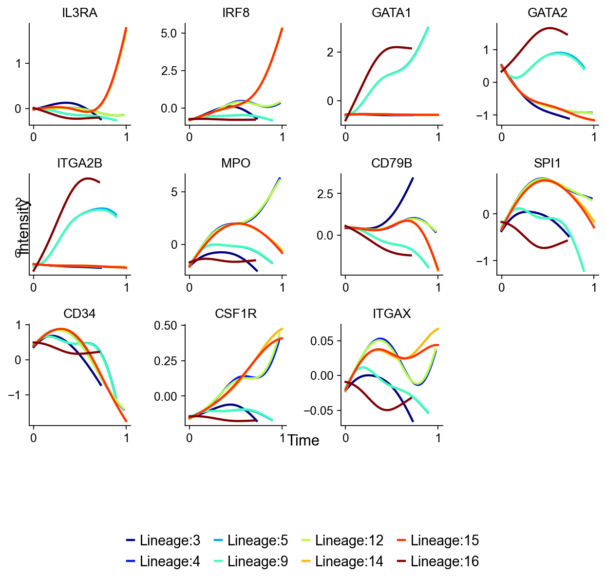
基因动态#
VIA 会自动沿检测到的谱系推断基因表达随伪时间变化的趋势。这些曲线可以理解为特定终末谱系上 marker 基因表达程序的动态变化。最后,我们再用热图汇总选定基因在指定谱系上的趋势。
fig,axs=v0.plot_gene_trend(gene_list=gene_list_magic,figsize=(8,6),)
fig.savefig('figures/via_fig8.png',dpi=300,bbox_inches = 'tight')
shape of transition matrix raised to power 3 (5780, 5780)
fig,ax=v0.plot_gene_trend_heatmap(
    gene_list=gene_list_magic,figsize=(4,4),
    marker_lineages=via_heatmap_lineages
)
fig.savefig('figures/via_fig9.png',dpi=300,bbox_inches = 'tight')
shape of transition matrix raised to power 3 (5780, 5780)