cNMF：共识非负矩阵分解

import scanpy as scimport omicverse as ovov.style(font_path='Arial')%load_ext autoreload%autoreload 2

🔬 Starting plot initialization...
Using already downloaded Arial font from: /tmp/omicverse_arial.ttf
Registered as: Arial
🧬 Detecting GPU devices…
✅ NVIDIA CUDA GPUs detected: 1
    • [CUDA 0] NVIDIA H100 80GB HBM3
      Memory: 79.1 GB | Compute: 9.0

   ____            _     _    __                  
  / __ \____ ___  (_)___| |  / /__  _____________ 
 / / / / __ `__ \/ / ___/ | / / _ \/ ___/ ___/ _ \ 
/ /_/ / / / / / / / /__ | |/ /  __/ /  (__  )  __/ 
\____/_/ /_/ /_/_/\___/ |___/\___/_/  /____/\___/                                              

🔖 Version: 1.7.9rc1   📚 Tutorials: https://omicverse.readthedocs.io/
✅ plot_set complete.

什么是cNMF？

adata=ov.datasets.pancreatic_endocrinogenesis()

🔍 Downloading data to ./data/endocrinogenesis_day15.h5ad
⚠️ File ./data/endocrinogenesis_day15.h5ad already exists
 Loading data from ./data/endocrinogenesis_day15.h5ad
✅ Successfully loaded: 3696 cells × 27998 genes

%%timeadata=ov.pp.preprocess(adata,mode='shiftlog|pearson',n_HVGs=2000,)adata

🔍 [2026-01-07 17:06:35] Running preprocessing in 'cpu' mode...
Begin robust gene identification
    After filtration, 17750/27998 genes are kept.
    Among 17750 genes, 16426 genes are robust.
✅ Robust gene identification completed successfully.
Begin size normalization: shiftlog and HVGs selection pearson

🔍 Count Normalization:
   Target sum: 500000.0
   Exclude highly expressed: True
   Max fraction threshold: 0.2
   ⚠️ Excluding 1 highly-expressed genes from normalization computation
   Excluded genes: ['Ghrl']

✅ Count Normalization Completed Successfully!
   ✓ Processed: 3,696 cells × 16,426 genes
   ✓ Runtime: 0.25s

🔍 Highly Variable Genes Selection (Experimental):
   Method: pearson_residuals
   Target genes: 2,000
   Theta (overdispersion): 100

✅ Experimental HVG Selection Completed Successfully!
   ✓ Selected: 2,000 highly variable genes out of 16,426 total (12.2%)
   ✓ Results added to AnnData object:
     • 'highly_variable': Boolean vector (adata.var)
     • 'highly_variable_rank': Float vector (adata.var)
     • 'highly_variable_nbatches': Int vector (adata.var)
     • 'highly_variable_intersection': Boolean vector (adata.var)
     • 'means': Float vector (adata.var)
     • 'variances': Float vector (adata.var)
     • 'residual_variances': Float vector (adata.var)
    Time to analyze data in cpu: 1.11 seconds.
✅ Preprocessing completed successfully.
    Added:
        'highly_variable_features', boolean vector (adata.var)
        'means', float vector (adata.var)
        'variances', float vector (adata.var)
        'residual_variances', float vector (adata.var)
        'counts', raw counts layer (adata.layers)
    End of size normalization: shiftlog and HVGs selection pearson
CPU times: user 1.43 s, sys: 717 ms, total: 2.15 s
Wall time: 1.51 s

AnnData object with n_obs × n_vars = 3696 × 16426
    obs: 'clusters_coarse', 'clusters', 'S_score', 'G2M_score'
    var: 'highly_variable_genes', 'n_cells', 'percent_cells', 'robust', 'highly_variable_features', 'means', 'variances', 'residual_variances', 'highly_variable_rank', 'highly_variable'
    uns: 'clusters_coarse_colors', 'clusters_colors', 'day_colors', 'neighbors', 'pca', 'log1p', 'hvg', 'status', 'status_args', 'REFERENCE_MANU'
    obsm: 'X_pca', 'X_umap'
    layers: 'spliced', 'unspliced', 'counts'
    obsp: 'distances', 'connectivities'

ov.pp.scale(adata)ov.pp.pca(adata)

computing PCA🔍
    with n_comps=50
   🖥️ Using sklearn PCA for CPU computation
   🖥️ sklearn PCA backend: CPU computation
    finished✅ (0:00:02)

# 导入库
import omicverse as ov
import scanpy as sc

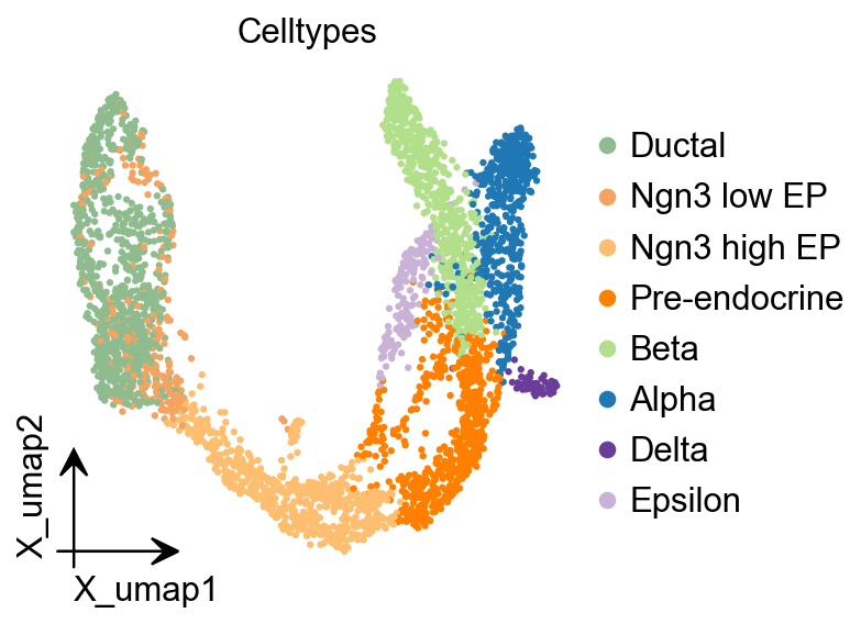
<Axes: title={'center': 'Celltypes'}, xlabel='X_umap1', ylabel='X_umap2'>

cNMF的工作原理

cNMF分解基因表达矩阵以识别基因模块和细胞类型。

# 准备数据
adata = ov.datasets.pbmc3k()
adata = ov.pp.preprocess(adata)

normalizing counts per cell
    finished (0:00:00)

# 运行cNMF
cnmf = ov.single.cNMF(adata)

🚀 Running NMF on GPU (device 0)
Running 200 factorization iterations for worker 0...
✓ Worker 0 completed 200 iterations. Total in memory: 200

参数选择

# 初始化cNMF
cnmf.initialize(K=10)

cnmf_obj.combine(skip_missing_files=True)

Combining factorizations for k=5.
  Found all 20 iterations for k=5
Combining factorizations for k=6.
  Found all 20 iterations for k=6
Combining factorizations for k=7.
  Found all 20 iterations for k=7
Combining factorizations for k=8.
  Found all 20 iterations for k=8
Combining factorizations for k=9.
  Found all 20 iterations for k=9
Combining factorizations for k=10.
  Found all 20 iterations for k=10
Combining factorizations for k=11.
  Found all 20 iterations for k=11
Combining factorizations for k=12.
  Found all 20 iterations for k=12
Combining factorizations for k=13.
  Found all 20 iterations for k=13
Combining factorizations for k=14.
  Found all 20 iterations for k=14

cnmf_obj.save('test/cnmf_obj.pkl')

✓ cNMF object saved to: test/cnmf_obj.pkl
  - 200 factorization iterations
  - 10 merged spectra (K values)
  - 0 consensus results

cnmf_obj.load('test/cnmf_obj.pkl')

📂 Load Operation:
   Source path: test/cnmf_obj.pkl
   Using: pickle
   ✅ Successfully loaded!
   Loaded object type: cNMF
────────────────────────────────────────────────────────────

cNMF工作流

sil_data = cnmf_obj.calculate_silhouette_k(k=7, density_threshold=2.0)print(f"Average silhouette score: {sil_data['avg_silhouette']:.4f}")print(f"Per-sample scores: {sil_data['silhouette_values']}")print(f"Cluster labels: {sil_data['cluster_labels']}")

Average silhouette score: 0.6299
Per-sample scores: [0.7106916  0.5630814  0.9380699  0.9647325  0.7674971  0.6231896
 0.7462224  0.37565622 0.6270655  0.06985006 0.57842237 0.7953116
 0.6916376  0.78109527 0.7101993  0.55603576 0.7441653  0.75451505
 0.5479283  0.9625558  0.39097318 0.43278462 0.97507685 0.60460097
 0.7781605  0.67471343 0.53983855 0.76693016 0.64284235 0.41358513
 0.7894957  0.5756324  0.9714798  0.54308915 0.73912    0.5916759
 0.29305577 0.5943038  0.9639678  0.75087273 0.4957365  0.7721111
 0.5499817  0.5790103  0.73023146 0.588068   0.77418405 0.18887511
 0.3828089  0.71155    0.93825644 0.66316015 0.7878561  0.9744356
 0.7274356  0.628735   0.96383363 0.63263124 0.64927    0.17515936
 0.7908563  0.59846324 0.67699015 0.37909067 0.7533861  0.27464965
 0.94846934 0.56372494 0.62612045 0.39772192 0.4309683  0.50130105
 0.5352081  0.2945753  0.7588943  0.7905221  0.7286009  0.94101614
 0.5963504  0.60703915 0.6570392  0.17053658 0.7238535  0.63654566
 0.164855   0.60783756 0.70025706 0.64824665 0.08693045 0.70052814
 0.6865447  0.5977072  0.95368004 0.7289692  0.44170102 0.7777483
 0.7743478  0.4995771  0.69891447 0.580345   0.78578705 0.3635015
 0.71654373 0.9585754  0.6125389  0.629792   0.6913672  0.4552708
 0.10541853 0.96240723 0.38784292 0.6745267  0.79051185 0.70214224
 0.84903276 0.6250461  0.509497   0.055472   0.6147614  0.49948195
 0.25953737 0.72868174 0.7900021  0.6660114  0.360943   0.6711156
 0.7861118  0.9580041  0.57364947 0.43281323 0.78196883 0.64617914
 0.50612485 0.1185286  0.7382589  0.9742657  0.67354196 0.76530886
 0.5728536  0.7114021 ]
Cluster labels: [4 2 0 6 3 1 5 1 2 4 1 3 4 5 4 2 5 3 1 0 1 1 6 2 5 4 1 3 2 1 3 4 6 1 5 1 1
 2 0 5 4 3 1 2 4 3 5 3 1 5 0 2 3 6 4 1 0 1 2 4 3 5 4 4 5 2 0 1 3 1 1 1 2 2
 5 3 4 6 1 5 2 3 4 3 3 1 5 2 4 3 4 2 0 4 1 3 5 1 5 1 3 1 4 0 2 1 3 5 2 0 2
 4 3 4 0 1 5 2 2 1 1 4 3 2 1 5 5 0 4 1 3 2 1 1 3 6 2 5 1 4]

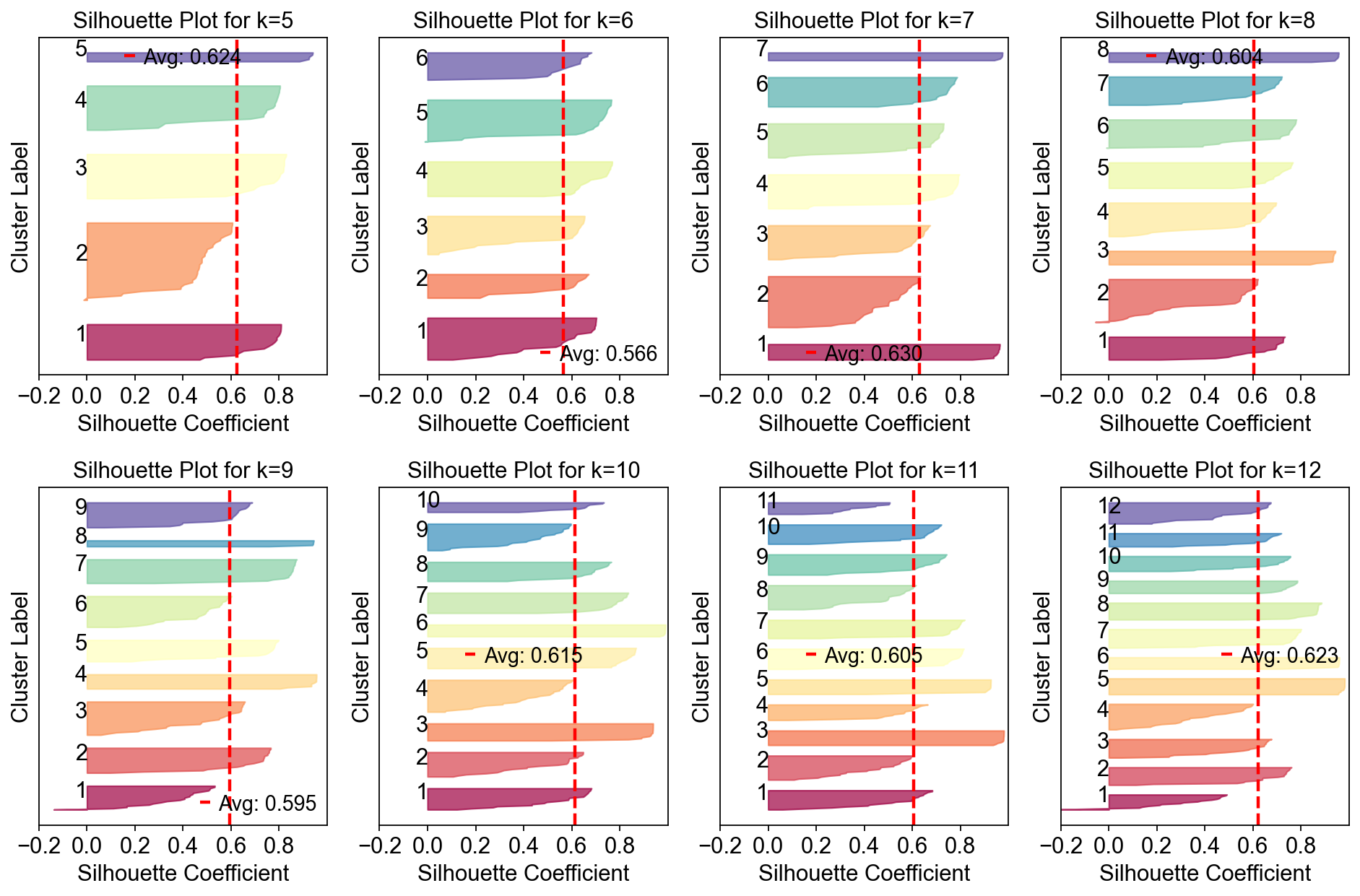
fig, axes = plt.subplots(2,4,figsize=(12,8))for k,ax in zip(np.arange(5,15),axes.flatten()):    cnmf_obj.plot_silhouette_for_k(        k=k,        density_threshold=2.0,        show_avg=True,        cmap='Spectral',ax=ax    )plt.tight_layout()

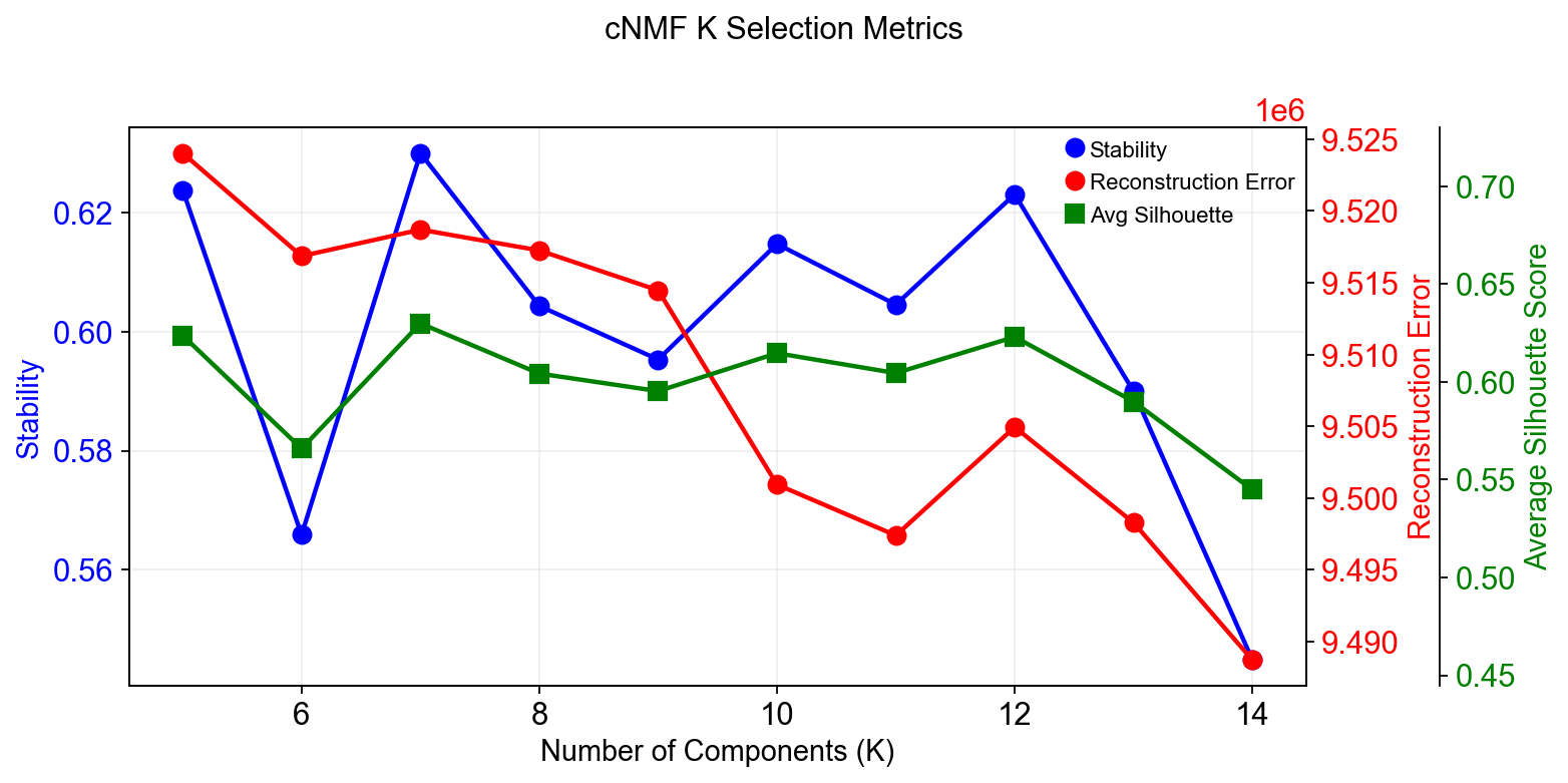
fig=cnmf_obj.k_selection_plot(close_fig=False)

Calculating silhouette scores for K selection...

结果解释

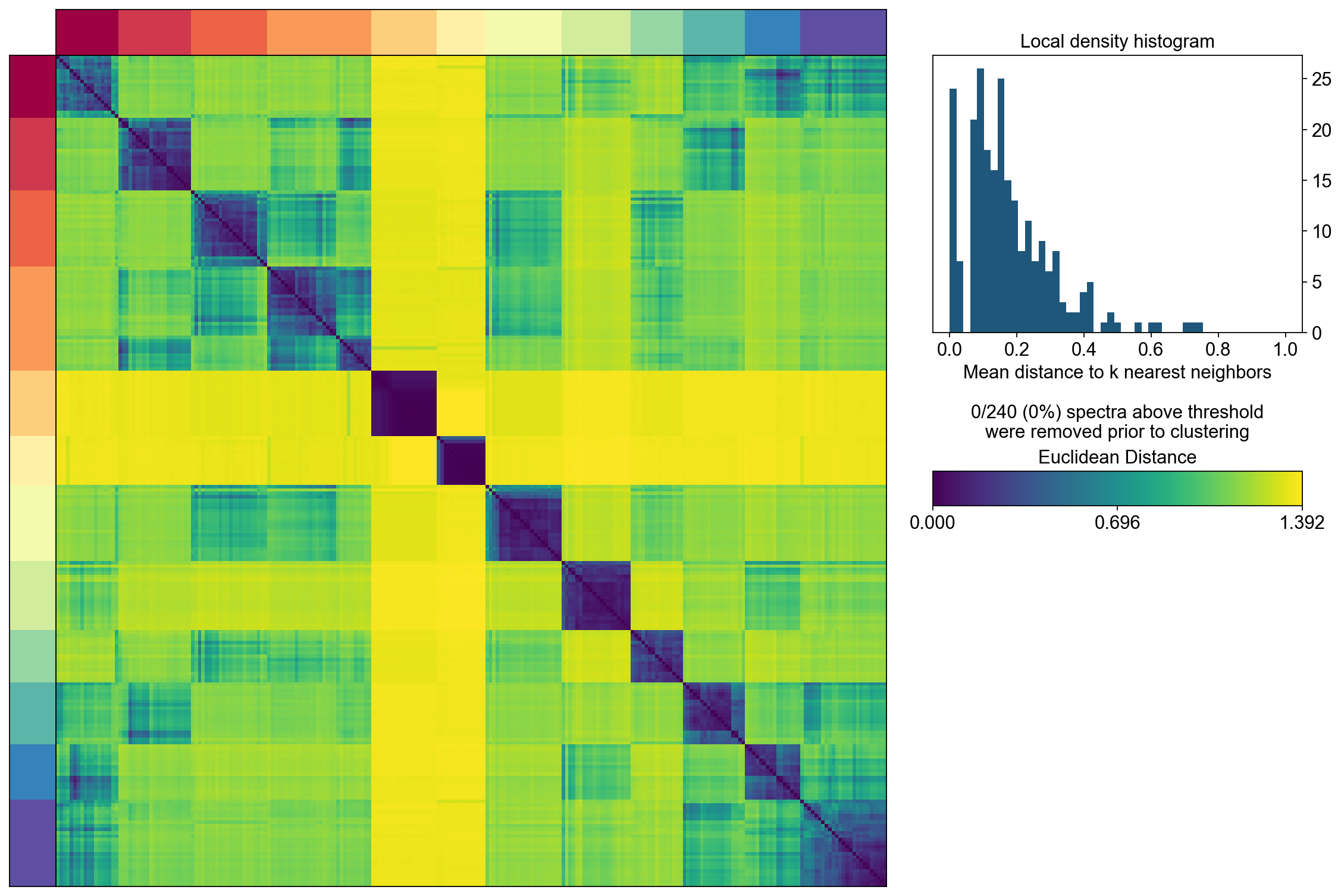
selected_K = 12density_threshold = 2.00

cnmf_obj.consensus(k=selected_K,                    density_threshold=density_threshold,                    show_clustering=True,                    close_clustergram_fig=False)

可视化

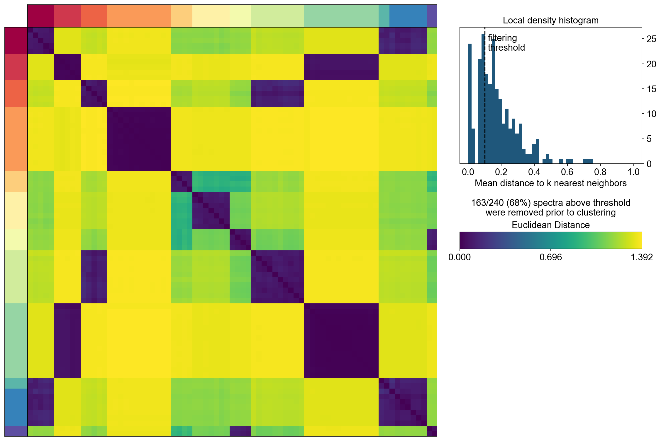
density_threshold = 0.10

cnmf_obj.consensus(k=selected_K,                    density_threshold=density_threshold,                    show_clustering=True,                    close_clustergram_fig=False)

继续分析

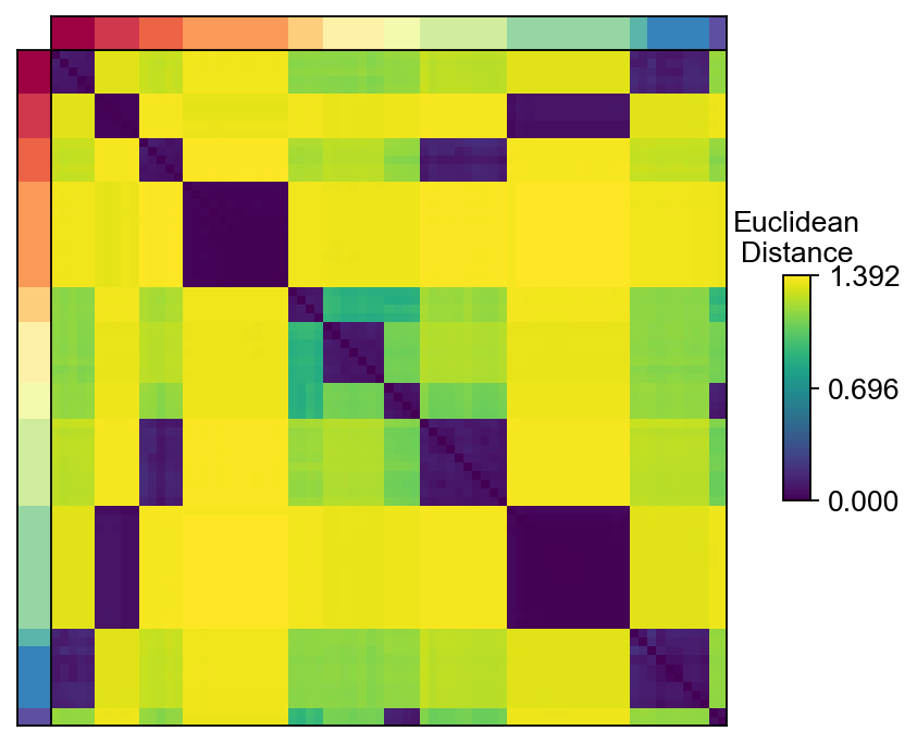
import seaborn as snsimport matplotlib.pyplot as pltfrom matplotlib import patheffectsfrom matplotlib import gridspecimport matplotlib.pyplot as pltwidth_ratios = [0.2, 4, 0.5, 10, 1]height_ratios = [0.2, 4]fig = plt.figure(figsize=(sum(width_ratios), sum(height_ratios)))gs = gridspec.GridSpec(len(height_ratios), len(width_ratios), fig,                        0.01, 0.01, 0.98, 0.98,                       height_ratios=height_ratios,                       width_ratios=width_ratios,                       wspace=0, hspace=0)            D = cnmf_obj.topic_dist[cnmf_obj.spectra_order, :][:, cnmf_obj.spectra_order]dist_ax = fig.add_subplot(gs[1,1], xscale='linear', yscale='linear',                                      xticks=[], yticks=[],xlabel='', ylabel='',                                      frameon=True)dist_im = dist_ax.imshow(D, interpolation='none', cmap='viridis',                         aspect='auto', rasterized=True)left_ax = fig.add_subplot(gs[1,0], xscale='linear', yscale='linear', xticks=[], yticks=[],                xlabel='', ylabel='', frameon=True)left_ax.imshow(cnmf_obj.kmeans_cluster_labels.values[cnmf_obj.spectra_order].reshape(-1, 1),                            interpolation='none', cmap='Spectral', aspect='auto',                            rasterized=True)top_ax = fig.add_subplot(gs[0,1], xscale='linear', yscale='linear', xticks=[], yticks=[],                xlabel='', ylabel='', frameon=True)top_ax.imshow(cnmf_obj.kmeans_cluster_labels.values[cnmf_obj.spectra_order].reshape(1, -1),                  interpolation='none', cmap='Spectral', aspect='auto',                    rasterized=True)cbar_gs = gridspec.GridSpecFromSubplotSpec(3, 3, subplot_spec=gs[1, 2],                                   wspace=0, hspace=0)cbar_ax = fig.add_subplot(cbar_gs[1,2], xscale='linear', yscale='linear',    xlabel='', ylabel='', frameon=True, title='Euclidean\nDistance')cbar_ax.set_title('Euclidean\nDistance',fontsize=12)vmin = D.min().min()vmax = D.max().max()fig.colorbar(dist_im, cax=cbar_ax,        ticks=np.linspace(vmin, vmax, 3),        )cbar_ax.set_yticklabels(cbar_ax.get_yticklabels(),fontsize=12)

[Text(1, 0.0, '0.000'),
 Text(1, 0.6961943507194519, '0.696'),
 Text(1, 1.3923887014389038, '1.392')]

# 提取和保存结果
results = cnmf.extract_results()
print(results)

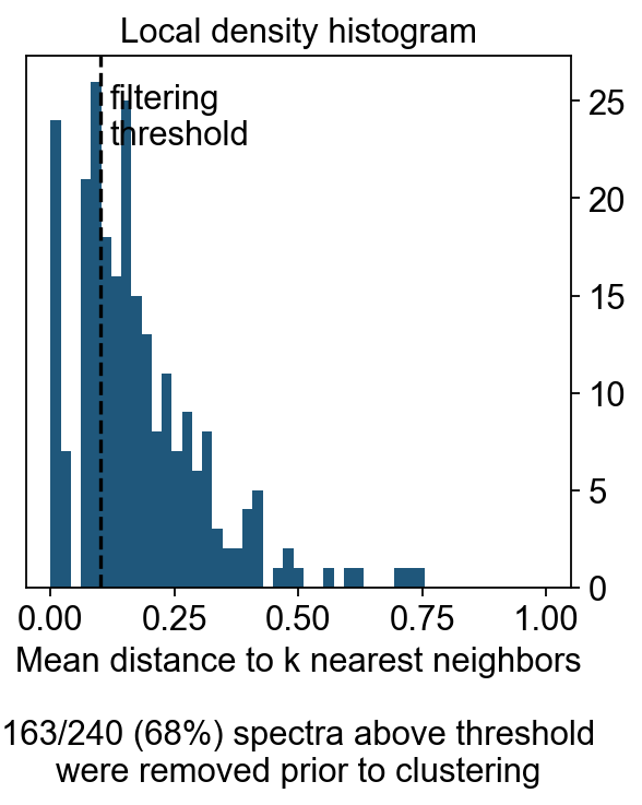
Text(0.5, 1.0, 'Local density histogram')

参数优化

result_dict = cnmf_obj.load_results(K=selected_K, density_threshold=density_threshold)

result_dict['usage_norm'].head()

	cNMF_1	cNMF_2	cNMF_3	cNMF_4	cNMF_5	cNMF_6	cNMF_7	cNMF_8	cNMF_9	cNMF_10	cNMF_11	cNMF_12
index
AAACCTGAGAGGGATA	0.052900	0.557367	0.000422	0.021016	0.006930	0.003447	0.079662	0.082491	0.000638	0.005284	0.030603	0.159242
AAACCTGAGCCTTGAT	0.020833	0.000962	0.570114	0.043898	0.000887	0.173351	0.007137	0.132107	0.004638	0.000670	0.029395	0.016007
AAACCTGAGGCAATTA	0.000142	0.306285	0.050380	0.000632	0.017096	0.028461	0.017249	0.053764	0.000810	0.005584	0.131687	0.387909
AAACCTGCATCATCCC	0.011620	0.000740	0.142481	0.011996	0.002794	0.510735	0.001547	0.281503	0.003506	0.025785	0.005863	0.001429
AAACCTGGTAAGTGGC	0.543322	0.149150	0.003397	0.199798	0.000105	0.011512	0.023303	0.000721	0.003200	0.022096	0.025705	0.017692

result_dict['gep_scores'].head()

	1	2	3	4	5	6	7	8	9	10	11	12
index
Xkr4	-0.007757	-0.001951	0.010988	0.000303	0.000153	-0.006076	0.001394	-0.000277	0.007163	-0.000909	-0.001658	-0.001580
Mrpl15	-0.004883	0.017592	-0.018511	-0.027615	-0.021772	0.037728	0.013916	0.011741	-0.016687	0.021974	-0.005451	-0.004443
Npbwr1	0.008097	0.001318	-0.010134	-0.018095	-0.016732	0.000294	-0.003005	0.000016	0.055294	-0.001144	-0.000746	-0.001143
4732440D04Rik	0.008619	-0.005695	-0.006195	-0.013188	0.014607	0.001333	-0.008327	-0.001492	0.005998	0.000943	0.000016	-0.002278
Gm26901	-0.007764	0.026168	-0.008942	0.023266	-0.009654	-0.017616	-0.010079	0.009438	-0.008486	-0.003649	-0.001237	-0.000615

result_dict['gep_tpm'].head()

	1	2	3	4	5	6	7	8	9	10	11	12
index
Xkr4	0.000000	8.302266e-03	1.477936e-02	0.000000	1.833748e-03	3.670955e-05	8.236001e-29	1.203458e-02	0.008952	0.000000	0.000000e+00	0.002387
Mrpl15	0.010844	4.420368e-19	9.274849e-01	0.018528	5.522656e-01	7.091711e-02	1.485689e-01	3.118949e-02	0.046750	0.155717	5.128206e-14	0.662705
Npbwr1	0.016931	0.000000e+00	2.428719e-16	0.000000	9.940618e-04	4.695393e-07	0.000000e+00	0.000000e+00	0.000000	0.009431	0.000000e+00	0.000000
4732440D04Rik	0.008692	1.156003e-05	7.946806e-03	0.000000	4.226314e-02	3.767684e-02	3.580834e-02	2.182026e-12	0.000063	0.005495	3.885308e-30	0.006224
Gm26901	0.000000	3.010304e-02	3.764709e-20	0.000000	1.401298e-45	1.688556e-03	8.005813e-03	0.000000e+00	0.000000	0.000000	0.000000e+00	0.062770

result_dict['top_genes'].head()

	1	2	3	4	5	6	7	8	9	10	11	12
0	Hmgn3	Anxa2	Nnat	Grin3a	Krt7	Sox4	Gmnn	Olfm1	Ghrl	Birc5	Prph	Gpr132
1	Chgb	Cldn3	Ppp1r1a	Atoh8	1110012L19Rik	Nptx2	Mcm5	Selm	Maged2	Nusap1	Stmn2	AB124611
2	Rap1b	Krt18	Ins2	Enpp2	BC023829	Mpzl1	Pcna	Ppp1r14a	Gm11837	Cenpf	Hand2	Tyrobp
3	Cldn4	Atp1b1	Sdf2l1	Ttr	Gspt1	Bcl2	2810417H13Rik	Tmsb4x	Arg1	Plk1	Stmn4	Fcgr3
4	Pax6	Lurap1l	Iapp	Tmem171	Cck	Gadd45a	Rrm2	Shf	Irs4	Cks2	Pirt	AI662270

跨数据集应用

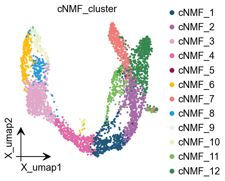
cnmf_obj.get_results(adata,result_dict)

cNMF_cluster is added to adata.obs
gene scores are added to adata.var

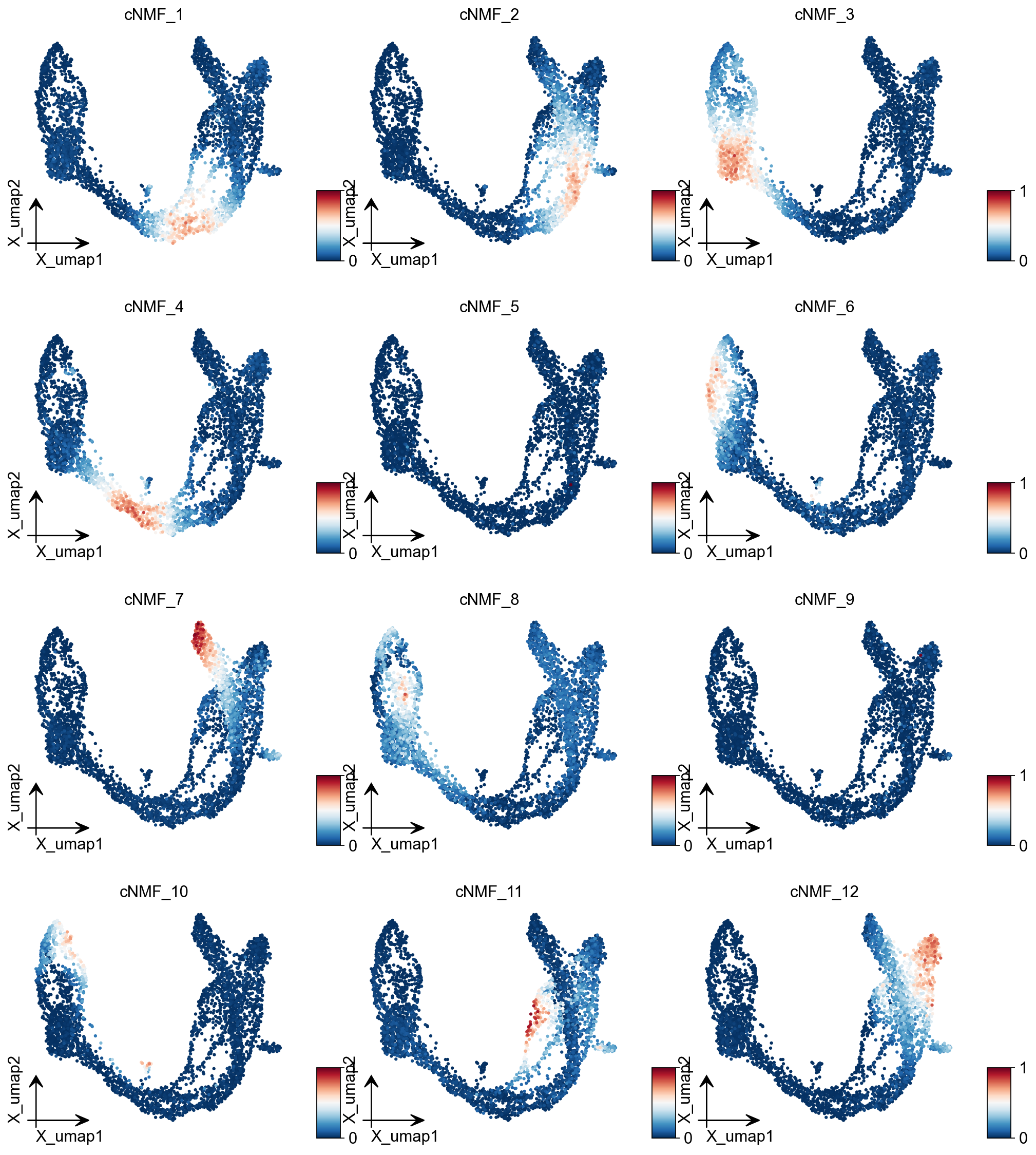
ov.pl.embedding(adata, basis='X_umap',color=result_dict['usage_norm'].columns,           use_raw=False, ncols=3, vmin=0, vmax=1,frameon='small')

# 比较多个K值
for k in range(5, 15):
    cnmf_k = ov.single.cNMF(adata, k=k)

<Axes: title={'center': 'cNMF_cluster'}, xlabel='X_umap1', ylabel='X_umap2'>

基因程序识别

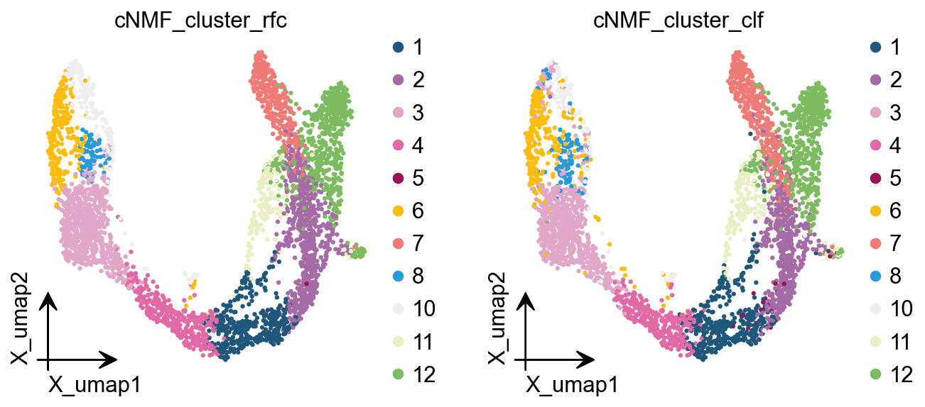
cnmf_obj.get_results_rfc(adata,result_dict,                         use_rep='scaled|original|X_pca',                        cNMF_threshold=0.5)

Single Tree: 0.9555555555555556
Random Forest: 0.9873015873015873
cNMF_cluster_rfc is added to adata.obs
cNMF_cluster_clf is added to adata.obs

# 识别基因程序
programs = cnmf.get_programs()

[<Axes: title={'center': 'cNMF_cluster_rfc'}, xlabel='X_umap1', ylabel='X_umap2'>,
 <Axes: title={'center': 'cNMF_cluster_clf'}, xlabel='X_umap1', ylabel='X_umap2'>]

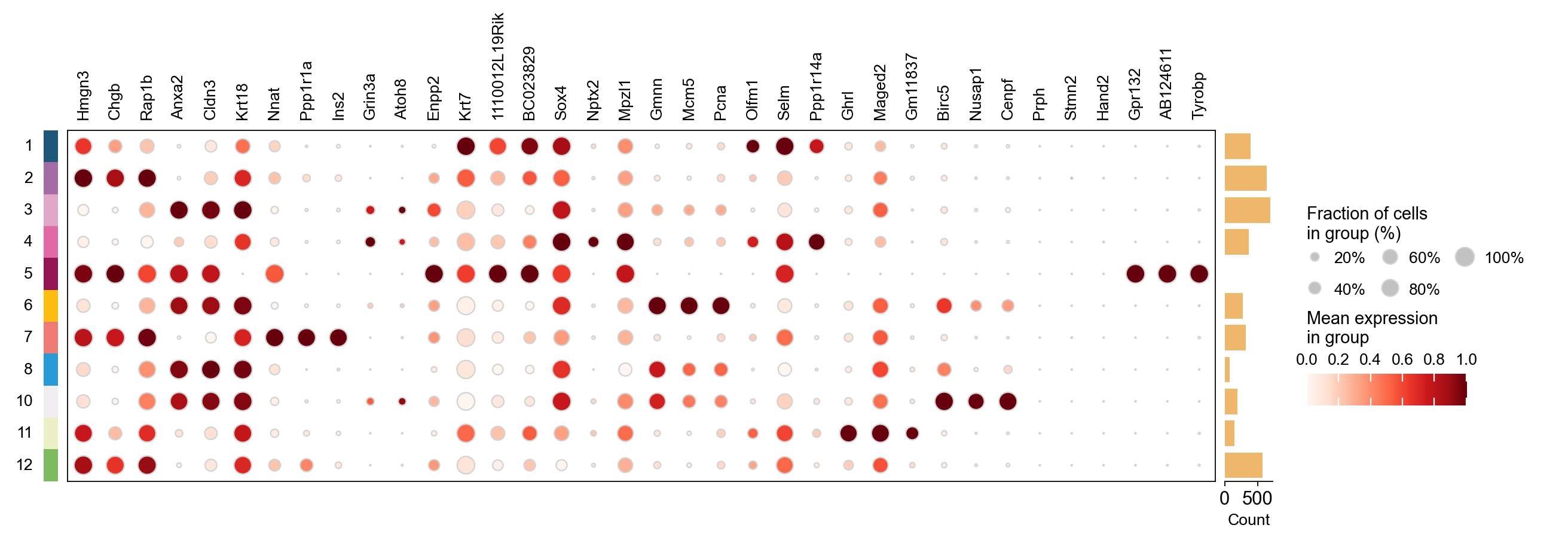
plot_genes=[]for i in result_dict['top_genes'].columns:    plot_genes+=result_dict['top_genes'][i][:3].values.reshape(-1).tolist()

ov.pl.dotplot(    adata,plot_genes,    "cNMF_cluster_rfc", dendrogram=False,standard_scale='var',)

<marsilea.heatmap.SizedHeatmap at 0x7f84d0263e20>

质量控制

# 评估cNMF质量
qc_metrics = cnmf.quality_control()

# 可视化质量指标
plot_data = pd.DataFrame(qc_metrics)

与其他方法的比较

hs_results = hs.compute_autocorrelations(jobs=8)hs_results.head(15)

	C	Z	Pval	FDR
Gene
Btbd17	0.735443	221.872382	0.0	0.0
Gadd45a	0.666501	213.692549	0.0	0.0
Neurog3	0.658402	208.855264	0.0	0.0
Spp1	0.806283	200.751152	0.0	0.0
Mdk	0.695210	199.681646	0.0	0.0
Rps19	0.819013	199.041836	0.0	0.0
Gnas	0.701187	192.850484	0.0	0.0
Rpl13	0.817551	192.250551	0.0	0.0
Nnat	0.780046	191.744472	0.0	0.0
Rpl18a	0.780471	191.128396	0.0	0.0
Rpl32	0.796391	190.960143	0.0	0.0
Gcg	0.603454	190.364941	0.0	0.0
Ins2	0.753340	189.588977	0.0	0.0
Ppp1r1a	0.727086	188.885836	0.0	0.0
Rps4x	0.797900	187.245979	0.0	0.0

高级应用

# 提取特定程序
program_genes = cnmf.get_program_genes(program_id=0)

Computing pair-wise local correlation on 500 features...

故障排除

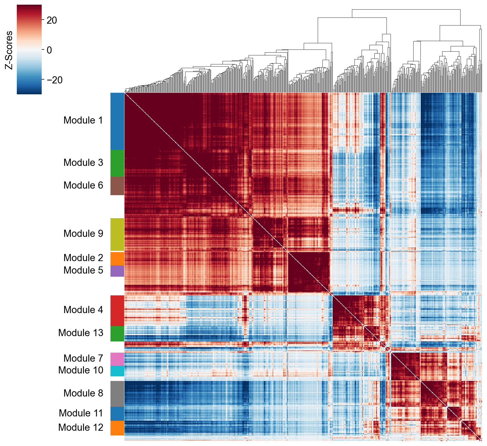
modules = hs.create_modules(    min_gene_threshold=15, core_only=True, fdr_threshold=0.05)modules.value_counts()

Module
-1     93
 1     82
 9     47
 4     44
 3     39
 8     37
 6     26
 13    22
 12    21
 11    20
 7     19
 2     19
 5     16
 10    15
Name: count, dtype: int64

hs.plot_local_correlations(vmin=-30, vmax=30,)

<seaborn.matrix.ClusterGrid at 0x7f52ab7e3f10>

进一步阅读

# 保存结果
cnmf.save_results(output_path='./cnmf_results')

	C	Z	Pval	FDR	Module
Gene
Btbd17	0.735443	221.872382	0.0	0.0	4.0
Gadd45a	0.666501	213.692549	0.0	0.0	4.0
Neurog3	0.658402	208.855264	0.0	0.0	4.0
Mdk	0.695210	199.681646	0.0	0.0	4.0
Tmsb4x	0.628210	187.142300	0.0	0.0	4.0
Neurod2	0.549973	183.843618	0.0	0.0	4.0
Selm	0.601179	178.700916	0.0	0.0	4.0
Smarcd2	0.577830	174.089181	0.0	0.0	4.0
Sox4	0.613079	173.945370	0.0	0.0	4.0
Btg2	0.554990	165.342505	0.0	0.0	4.0

总结

module_scores = hs.calculate_module_scores()module_scores.head()

Computing scores for 13 modules...

	1	2	3	4	5	6	7	8	9	10	11	12	13
index
AAACCTGAGAGGGATA	-6.583796	-1.093584	-3.131375	-2.099180	-0.819142	-2.400016	-0.451105	2.504838	-2.298986	-1.439230	-0.739708	3.368700	0.531080
AAACCTGAGCCTTGAT	7.663903	-0.765588	6.610663	-2.388122	-0.689135	2.296545	-1.217827	-3.391921	0.921212	-0.813991	-1.694216	-2.358554	-2.625691
AAACCTGAGGCAATTA	-6.066218	-1.212847	-3.005648	-2.684893	-0.703958	-2.226183	-0.702572	2.636014	-2.243965	-0.119376	0.899747	2.736469	-0.274772
AAACCTGCATCATCCC	11.594423	4.786089	5.015609	-2.241397	0.848967	8.482152	-0.886003	-3.327994	12.943623	0.456323	-1.689177	-2.565122	-2.858705
AAACCTGGTAAGTGGC	-3.090054	-1.036188	-3.197947	5.563916	-0.793746	-2.413544	-1.378844	-2.149192	-2.072845	-2.134279	-1.460957	-0.137338	6.417286

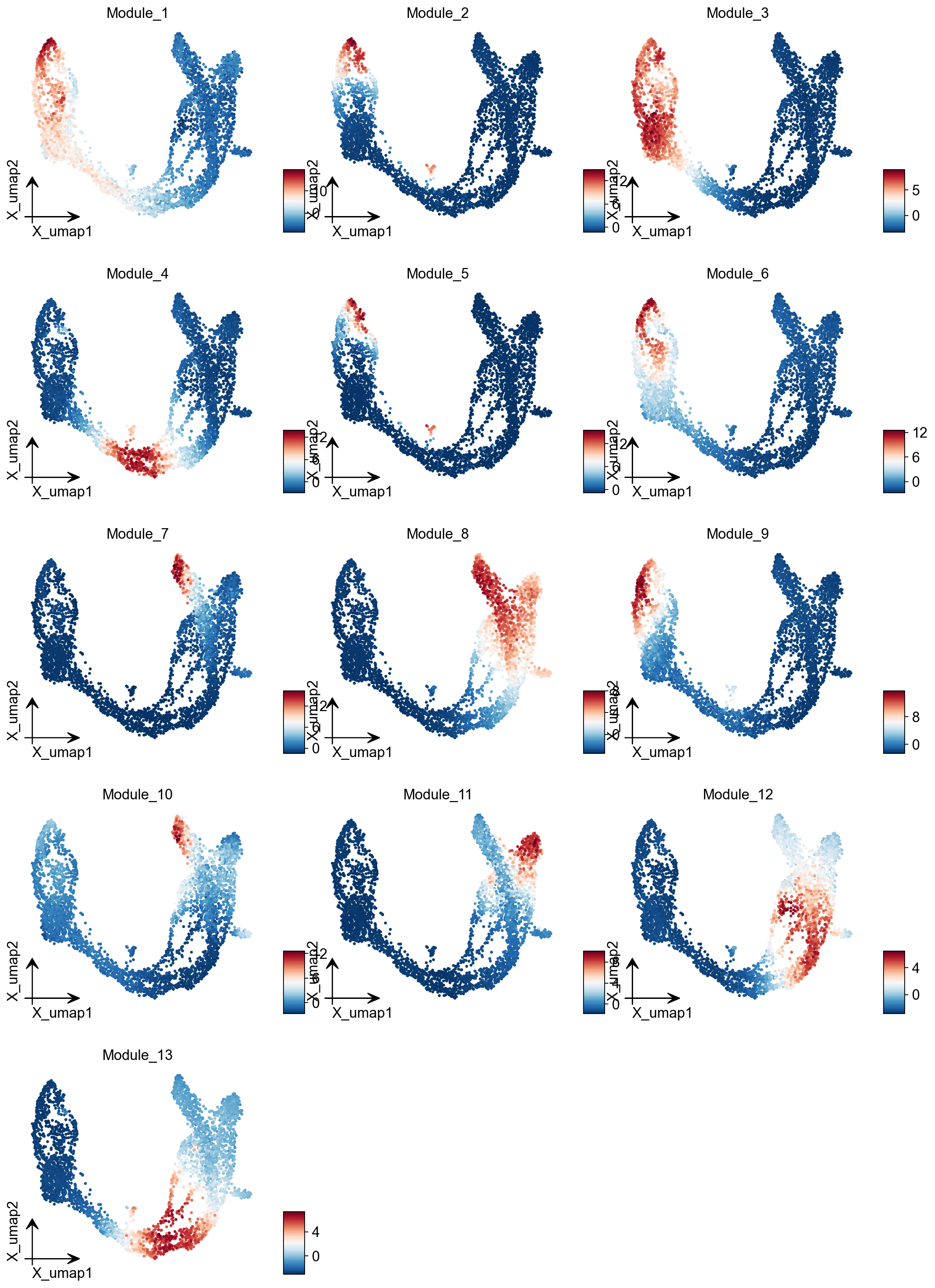
module_cols = []for c in module_scores.columns:    key = f"Module_{c}"    adata.obs[key] = module_scores[c]    module_cols.append(key)

ov.pl.embedding(adata, basis='X_umap',color=module_cols,           use_raw=False, ncols=3, frameon='small')