Bulk RNA-seq或微阵列数据中的批次校正#
数据集中的变异性不仅是生物学过程的产物,也是技术偏差的产物(Lander等,1999年)。ComBat是最广泛使用的批次效应校正工具之一,用于纠正这些被称为批次效应的技术偏差。
pyComBat(Behdenna等,2020年)是ComBat(Johnson等,2007年)的一个新的Python实现,ComBat是一款广泛用于微阵列数据批次效应校正的软件。虽然数学框架完全相同,但pyComBat:
在批次效应校正方面具有类似的结果;
速度与R版本的ComBat相当或更快;
为社区提供了参与其开发的新工具。
Code: epigenelabs/pyComBat
Colab_Reproducibility:https://colab.research.google.com/drive/121bbIiI3j4pTZ3yA_5p8BRkRyGMMmNAq?usp=sharing
import anndata
import pandas as pd
import omicverse as ov
ov.ov_plot_set()
AnnData object with n_obs × n_vars = 17126 × 161
Loading dataset#
This minimal usage example illustrates how to use pyComBat in a default setting, and shows some results on ovarian cancer data, freely available on NCBI’s Gene Expression Omnibus, namely:
GSE18520
GSE66957
GSE69428
The corresponding expression files are available on GitHub.
dataset_1 = pd.read_pickle("data/combat/GSE18520.pickle")
adata1=anndata.AnnData(dataset_1.T)
adata1.obs['batch']='1'
adata1
AnnData object with n_obs × n_vars = 63 × 21755
    obs: 'batch'
dataset_2 = pd.read_pickle("data/combat/GSE66957.pickle")
adata2=anndata.AnnData(dataset_2.T)
adata2.obs['batch']='2'
adata2
AnnData object with n_obs × n_vars = 69 × 22115
    obs: 'batch'
dataset_3 = pd.read_pickle("data/combat/GSE69428.pickle")
adata3=anndata.AnnData(dataset_3.T)
adata3.obs['batch']='3'
adata3
AnnData object with n_obs × n_vars = 29 × 21755
    obs: 'batch'
我们使用concat函数将三个数据集合并,并取相同基因的交集。
adata=anndata.concat([adata1,adata2,adata3],merge='same')
adata
AnnData object with n_obs × n_vars = 161 × 17126
    obs: 'batch'
去除批次效应#
ov.bulk.batch_correction(adata,batch_key='batch')
Found 3 batches.
Adjusting for 0 covariate(s) or covariate level(s).
Standardizing Data across genes.
Fitting L/S model and finding priors.
Finding parametric adjustments.
Adjusting the Data
Storing batch correction result in adata.layers['batch_correction']
保存结果#
原始数据集
raw_data=adata.to_df().T
raw_data.head()
| GSM461348 | GSM461349 | GSM461350 | GSM461351 | GSM461352 | GSM461353 | GSM461354 | GSM461355 | GSM461356 | GSM461357 | ... | GSM1701044 | GSM1701045 | GSM1701046 | GSM1701047 | GSM1701048 | GSM1701049 | GSM1701050 | GSM1701051 | GSM1701052 | GSM1701053 | |
|---|---|---|---|---|---|---|---|---|---|---|---|---|---|---|---|---|---|---|---|---|---|
| gene_symbol | |||||||||||||||||||||
| A1BG | 4.140079 | 4.589471 | 4.526200 | 4.326366 | 4.141506 | 4.528423 | 4.419378 | 4.345215 | 4.184150 | 4.393646 | ... | 3.490229 | 4.542913 | 4.654638 | 4.199212 | 4.080964 | 4.114272 | 3.883770 | 4.103220 | 3.883770 | 3.487520 |
| A1BG-AS1 | 5.747137 | 6.130257 | 5.781449 | 5.914044 | 6.277715 | 5.668244 | 5.879830 | 6.013979 | 5.968187 | 6.017624 | ... | 4.005230 | 4.301880 | 4.509698 | 4.089223 | 4.129560 | 3.867568 | 4.094032 | 3.616044 | 4.307225 | 3.891060 |
| A1CF | 5.026369 | 5.120523 | 5.220462 | 4.828303 | 5.078094 | 5.204209 | 4.865024 | 5.119230 | 5.219517 | 4.706891 | ... | 4.225589 | 3.530307 | 3.215182 | 2.967515 | 3.012953 | 3.496765 | 3.117002 | 3.072093 | 2.570765 | 3.163533 |
| A2M | 7.892506 | 7.730116 | 7.796338 | 8.525167 | 7.545033 | 7.846979 | 7.638513 | 7.487679 | 7.533089 | 6.965395 | ... | 10.273206 | 4.061912 | 4.393332 | 4.716536 | 3.447348 | 3.134037 | 4.009413 | 3.953612 | 7.664853 | 3.548574 |
| A2ML1 | 3.966217 | 4.482255 | 3.964664 | 3.906967 | 3.952821 | 3.985276 | 3.997008 | 4.101457 | 4.015285 | 3.765736 | ... | 2.478731 | 4.132282 | 3.952693 | 2.527621 | 2.358378 | 2.414869 | 2.204600 | 2.295500 | 2.167646 | 2.216867 |
5 rows × 161 columns
批次校正后的数据集
removing_data=adata.to_df(layer='batch_correction').T
removing_data.head()
| GSM461348 | GSM461349 | GSM461350 | GSM461351 | GSM461352 | GSM461353 | GSM461354 | GSM461355 | GSM461356 | GSM461357 | ... | GSM1701044 | GSM1701045 | GSM1701046 | GSM1701047 | GSM1701048 | GSM1701049 | GSM1701050 | GSM1701051 | GSM1701052 | GSM1701053 | |
|---|---|---|---|---|---|---|---|---|---|---|---|---|---|---|---|---|---|---|---|---|---|
| gene_symbol | |||||||||||||||||||||
| A1BG | 4.223549 | 4.846659 | 4.758930 | 4.481847 | 4.225527 | 4.762011 | 4.610814 | 4.507982 | 4.284656 | 4.575134 | ... | 4.237836 | 5.378695 | 5.499778 | 5.006204 | 4.878052 | 4.914150 | 4.664341 | 4.902172 | 4.664341 | 4.234900 |
| A1BG-AS1 | 5.730287 | 6.253722 | 5.777166 | 5.958322 | 6.455185 | 5.622501 | 5.911578 | 6.094858 | 6.032295 | 6.099838 | ... | 5.841898 | 5.990944 | 6.095359 | 5.884098 | 5.904365 | 5.772731 | 5.886515 | 5.646358 | 5.993630 | 5.784535 |
| A1CF | 3.922941 | 3.975597 | 4.031489 | 3.812171 | 3.951869 | 4.022399 | 3.832708 | 3.974874 | 4.030960 | 3.744271 | ... | 4.229097 | 3.822095 | 3.637628 | 3.492649 | 3.519248 | 3.802460 | 3.580155 | 3.553867 | 3.260401 | 3.607394 |
| A2M | 9.488789 | 9.219466 | 9.329295 | 10.538060 | 8.912504 | 9.413282 | 9.067542 | 8.817383 | 8.892696 | 7.951175 | ... | 11.137033 | 7.182184 | 7.393206 | 7.598996 | 6.790880 | 6.591389 | 7.148757 | 7.113228 | 9.476245 | 6.855333 |
| A2ML1 | 4.317770 | 5.553678 | 4.314051 | 4.175866 | 4.285686 | 4.363418 | 4.391514 | 4.641670 | 4.435287 | 3.837621 | ... | 3.807064 | 5.766146 | 5.553374 | 3.864987 | 3.664473 | 3.731402 | 3.482281 | 3.589976 | 3.438499 | 3.496814 |
5 rows × 161 columns
保存
raw_data.to_csv('raw_data.csv')
removing_data.to_csv('removing_data.csv')
您也可以保存adata对象
adata.write_h5ad('adata_batch.h5ad',compression='gzip')
#adata=ov.read('adata_batch.h5ad')
比较校正前后的数据集#
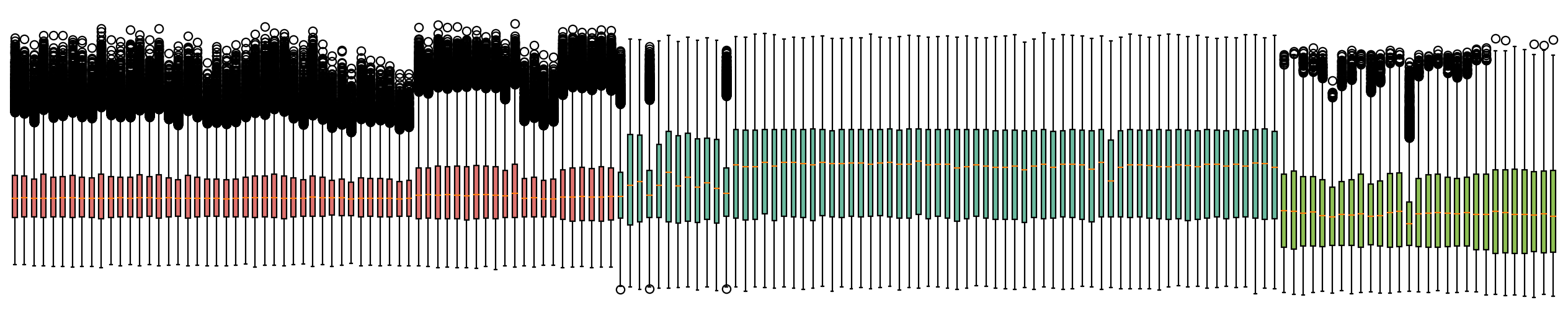
我们为三个不同的数据集指定三种不同的颜色
color_dict={
    '1':ov.utils.red_color[1],
    '2':ov.utils.blue_color[1],
    '3':ov.utils.green_color[1],
}
fig,ax=plt.subplots( figsize = (20,4))
bp=plt.boxplot(adata.to_df().T,patch_artist=True)
for i,batch in zip(range(adata.shape[0]),adata.obs['batch']):
    bp['boxes'][i].set_facecolor(color_dict[batch])
ax.axis(False)
plt.show()
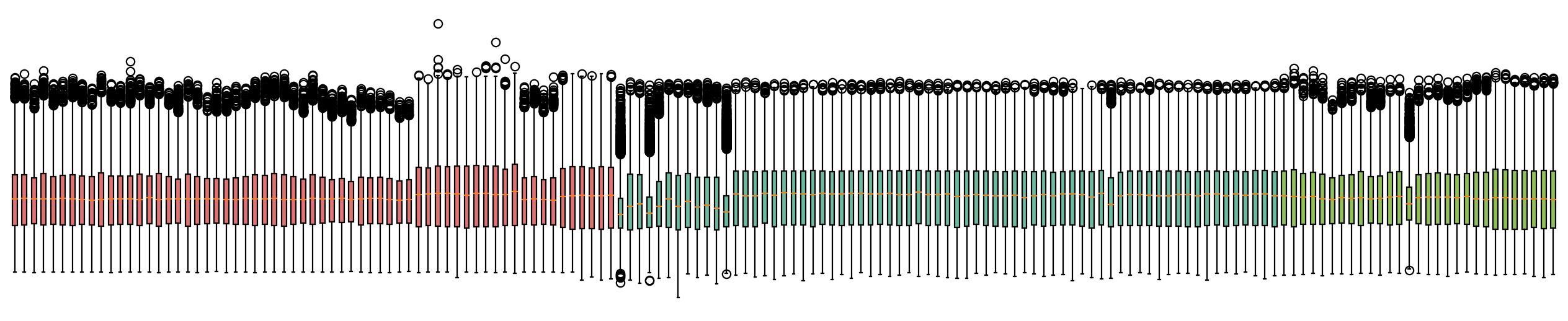
fig,ax=plt.subplots( figsize = (20,4))
bp=plt.boxplot(adata.to_df(layer='batch_correction').T,patch_artist=True)
for i,batch in zip(range(adata.shape[0]),adata.obs['batch']):
    bp['boxes'][i].set_facecolor(color_dict[batch])
ax.axis(False)
plt.show()
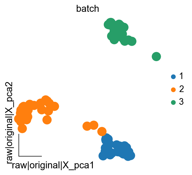
除了使用箱线图观察批次去除效果外,我们还可以使用PCA来观察批次去除的效果。
adata.layers['raw']=adata.X.copy()
我们首先对原始数据集计算PCA。
ov.pp.pca(adata,layer='raw',n_pcs=50)
adata
AnnData object with n_obs × n_vars = 161 × 17126
    obs: 'batch'
    uns: 'raw|original|pca_var_ratios', 'raw|original|cum_sum_eigenvalues'
    obsm: 'raw|original|X_pca'
    varm: 'raw|original|pca_loadings'
    layers: 'batch_correction', 'raw', 'lognorm'
然后我们对批次校正后的数据集计算PCA。
ov.pp.pca(adata,layer='batch_correction',n_pcs=50)
adata
AnnData object with n_obs × n_vars = 161 × 17126
    obs: 'batch'
    uns: 'raw|original|pca_var_ratios', 'raw|original|cum_sum_eigenvalues', 'batch_correction|original|pca_var_ratios', 'batch_correction|original|cum_sum_eigenvalues'
    obsm: 'raw|original|X_pca', 'batch_correction|original|X_pca'
    varm: 'raw|original|pca_loadings', 'batch_correction|original|pca_loadings'
    layers: 'batch_correction', 'raw', 'lognorm'
ov.pl.embedding(adata,
                  basis='raw|original|X_pca',
                  color='batch',
                  frameon='small')
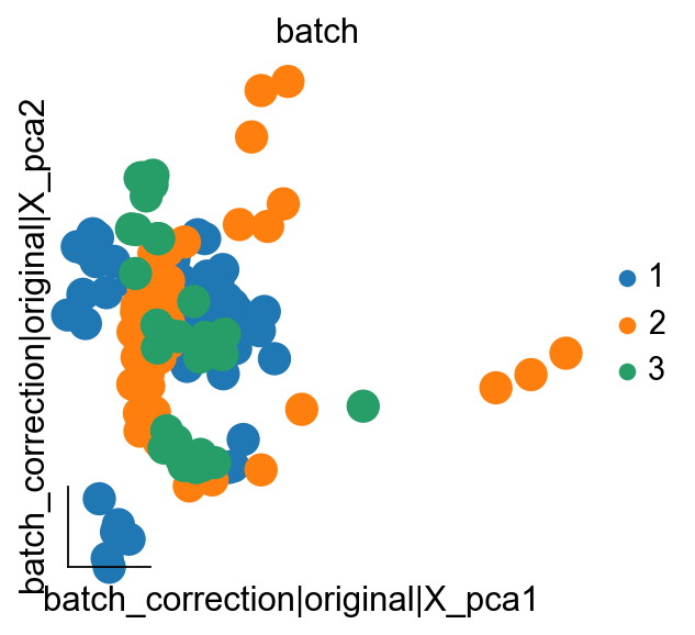
ov.pl.embedding(adata,
                  basis='batch_correction|original|X_pca',
                  color='batch',
                  frameon='small')