使用 CellPhoneDB 进行细胞通讯分析#
概览#
本教程围绕 OmicVerse 中的 CellPhoneDB 工作流展开,并使用同一套 ccc_* 接口组织所有可视化。
本教程按三类视图展开:
ov.pl.ccc_heatmapov.pl.ccc_network_plotov.pl.ccc_stat_plot
目的不是简单罗列图形,而是让你知道:
哪些图适合看 interaction 细节
哪些图适合看 pathway 聚合
哪些图适合做网络解释和优先级筛选
方法背景#
参考 CellPhoneDB 官方文档 和更新后的 CellPhoneDB v5 Nature Protocols 文章,CellPhoneDB 关注配体-受体介导的细胞通讯,并显式考虑 multimeric complex 的组合关系。
它的核心流程可以概括为:
准备标准化表达矩阵和细胞类型注释表
为每个 sender-receiver 组合计算 interaction mean
通过置换细胞标签来判断哪些 interaction mean 具有超出随机背景的特异性
将显著的相互作用进一步汇总到 pathway 和 network 层面进行解释
这种基于 permutation 的设计很重要,因为它可以把“表达量高但并不特异”的信号,与“真正偏向某些细胞类型组合”的通讯轴区分开来。
为什么这里使用 EVT 数据?#
这套 EVT 滋养层数据是 CellPhoneDB 示例里非常常见的数据集,包含比较容易解释的 trophoblast-immune 相互作用,因此很适合拿来演示如何把 interaction-level 结果进一步组织成更高层次的通讯视图。
import numpy as np
import pandas as pd
import scanpy as sc
import warnings
warnings.filterwarnings("ignore", category=FutureWarning)

import omicverse as ov

ov.plot_set(font_path='Arial')

%reload_ext autoreload
%autoreload 2
🔬 Starting plot initialization...
Using already downloaded Arial font from: /var/folders/rv/3jnfbs0d6r7d0c5bfj7ft5k00000gn/T/omicverse_arial.ttf
Registered as: Arial
🧬 Detecting GPU devices…
✅ Apple Silicon MPS detected
    • [MPS] Apple Silicon GPU - Metal Performance Shaders available

   ____            _     _    __
  / __ \____ ___  (_)___| |  / /__  _____________
 / / / / __ `__ \/ / ___/ | / / _ \/ ___/ ___/ _ \
/ /_/ / / / / / / / /__ | |/ /  __/ /  (__  )  __/
\____/_/ /_/ /_/_/\___/ |___/\___/_/  /____/\___/

🔖 Version: 2.1.3rc1   📚 Tutorials: https://omicverse.readthedocs.io/
✅ plot_set complete.
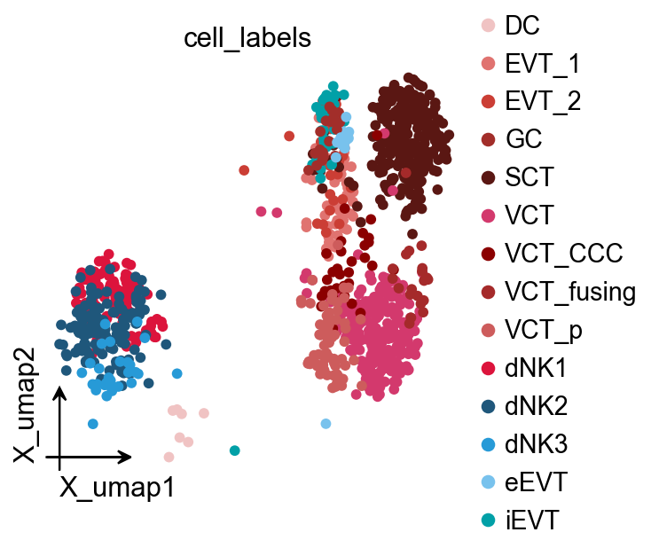
1. 载入 EVT 数据#
这里使用 CellPhoneDB 官方教程常见的 EVT 数据。
这一步的目标是:
准备表达矩阵
准备细胞类型注释
为后续 CellPhoneDB /
ccc_*示例提供统一输入
adata = ov.read('data/cpdb/normalised_log_counts.h5ad')
adata = adata[
    adata.obs['cell_labels'].isin(
        [
            'eEVT', 'iEVT', 'EVT_1', 'EVT_2', 'DC',
            'dNK1', 'dNK2', 'dNK3', 'VCT', 'VCT_CCC',
            'VCT_fusing', 'VCT_p', 'GC', 'SCT',
        ]
    )
]
adata
View of AnnData object with n_obs × n_vars = 1065 × 30800
    obs: 'n_genes', 'n_counts', 'cell_labels'
    var: 'gene_ids', 'feature_types'
    uns: 'neighbors_scVI_n_latent_14_sample_n_layers_3', 'neighbors_scVI_n_latent_20_sample_n_layers_3', 'umap'
    obsm: 'X_scVI_n_latent_14_sample_n_layers_3', 'X_scVI_n_latent_20_sample_n_layers_3', 'X_umap', 'X_umap_scVI_n_latent_14_sample_n_layers_3', 'X_umap_scVI_n_latent_20_sample_n_layers_3'
    obsp: 'neighbors_scVI_n_latent_14_sample_n_layers_3_connectivities', 'neighbors_scVI_n_latent_14_sample_n_layers_3_distances', 'neighbors_scVI_n_latent_20_sample_n_layers_3_connectivities', 'neighbors_scVI_n_latent_20_sample_n_layers_3_distances'
ov.pl.embedding(
    adata,
    basis='X_umap',
    color='cell_labels',
    frameon='small',
    palette=ov.pl.red_color + ov.pl.blue_color + ov.pl.green_color + ov.pl.orange_color + ov.pl.purple_color,
)
2. 运行 CellPhoneDB#
ov.single.run_cellphonedb_v5(...) 会返回:
cpdb_results:原始结果表adata_cpdb:标准通信AnnData
同时,也会把结果写回原始 adata.uns['cpdb_results'],因此后续 ccc_* 可以直接消费原始 adata。
cpdb_results, adata_cpdb = ov.single.run_cellphonedb_v5(
    adata,
    cpdb_file_path='./cellphonedb.zip',
    celltype_key='cell_labels',
    min_cell_fraction=0.005,
    min_genes=200,
    min_cells=3,
    iterations=1000,
    threshold=0.1,
    pvalue=0.05,
    threads=10,
    output_dir='./cpdb_results',
    cleanup_temp=True,
)
🔬 Starting CellPhoneDB analysis...
✅ Valid CellPhoneDB database found: ./cellphonedb.zip (0.1 MB)
   - Original data: 1065 cells, 30800 genes
   - Cell types passing 0.5% threshold: 14
   - Minimum cells required: 5
   - After filtering: 1065 cells, 30800 genes
- After preprocessing: 1065 cells, 19642 genes
   - Temporary directory: /var/folders/rv/3jnfbs0d6r7d0c5bfj7ft5k00000gn/T/cpdb_temp_2inw2pw9
   - Output directory: ./cpdb_results
- Created temporary input files
   - Running CellPhoneDB statistical analysis...
Reading user files...
The following user files were loaded successfully:
/var/folders/rv/3jnfbs0d6r7d0c5bfj7ft5k00000gn/T/cpdb_temp_2inw2pw9/counts_matrix.h5ad
/var/folders/rv/3jnfbs0d6r7d0c5bfj7ft5k00000gn/T/cpdb_temp_2inw2pw9/metadata.tsv
[ ][CORE][25/04/26-11:15:09][INFO] [Cluster Statistical Analysis] Threshold:0.1 Iterations:1000 Debug-seed:42 Threads:10 Precision:3
[ ][CORE][25/04/26-11:15:09][WARNING] Debug random seed enabled. Set to 42
[ ][CORE][25/04/26-11:15:09][INFO] Running Real Analysis
[ ][CORE][25/04/26-11:15:09][INFO] Running Statistical Analysis
[ ][CORE][25/04/26-11:15:13][INFO] Building Pvalues result
[ ][CORE][25/04/26-11:15:14][INFO] Building results
[ ][CORE][25/04/26-11:15:14][INFO] Scoring interactions: Filtering genes per cell type..
[ ][CORE][25/04/26-11:15:14][INFO] Scoring interactions: Calculating mean expression of each gene per group/cell type..
[ ][CORE][25/04/26-11:15:14][INFO] Scoring interactions: Calculating scores for all interactions and cell types..
Saved deconvoluted to ./cpdb_results/statistical_analysis_deconvoluted_04_25_2026_111524.txt
Saved deconvoluted_percents to ./cpdb_results/statistical_analysis_deconvoluted_percents_04_25_2026_111524.txt
Saved means to ./cpdb_results/statistical_analysis_means_04_25_2026_111524.txt
Saved pvalues to ./cpdb_results/statistical_analysis_pvalues_04_25_2026_111524.txt
Saved significant_means to ./cpdb_results/statistical_analysis_significant_means_04_25_2026_111524.txt
Saved interaction_scores to ./cpdb_results/statistical_analysis_interaction_scores_04_25_2026_111524.txt
   - CellPhoneDB analysis completed successfully!
   - Formatting results for visualization...
   - Found 13 info columns and 196 cell type pairs
   - Found 121 pathway classifications
   - Created visualization AnnData: (196, 1441)
   - Cell interactions: 196
   - L-R pairs: 1441
   - Cleaned up temporary directory: /var/folders/rv/3jnfbs0d6r7d0c5bfj7ft5k00000gn/T/cpdb_temp_2inw2pw9
✅ CellPhoneDB analysis pipeline completed!
如果你已经提前保存过结果,也可以直接加载缓存,而不重新跑 CellPhoneDB。
# cpdb_results = ov.utils.load('data/cpdb/gex_cpdb_test.pkl')
# adata_cpdb = ov.read('data/cpdb/gex_cpdb_ad.h5ad')
3. 准备下游绘图对象和辅助变量#
这里统一准备:
adata_plot:优先使用原始adata(如果已写入cpdb_results),否则退回adata_cpdbcomm_adata:显式提取的标准通信对象,便于差异示例和高级图color_dict/node_positions/embedding_points:网络图常用辅助信息
if 'cell_labels_colors' not in adata.uns:
    fallback_colors = (
        ov.pl.red_color
        + ov.pl.blue_color
        + ov.pl.green_color
        + ov.pl.orange_color
        + ov.pl.purple_color
    )
    adata.uns['cell_labels_colors'] = fallback_colors[:len(adata.obs['cell_labels'].cat.categories)]

color_dict = dict(zip(
    adata.obs['cell_labels'].cat.categories,
    adata.uns['cell_labels_colors']
))

adata_plot = adata if 'cpdb_results' in adata.uns else adata_cpdb
comm_adata = ov.single.extract_comm_adata(adata, result_uns_key='cpdb_results') if 'cpdb_results' in adata.uns else adata_cpdb

focus_pathway = 'Signaling by Fibroblast growth factor'
focus_pair_lr = 'NCAM1_FGFR1'
focus_ligand = 'FN1'

umap_df = pd.DataFrame(
    adata.obsm['X_umap'][:, :2],
    columns=['x', 'y'],
    index=adata.obs_names,
)
umap_df['cell_type'] = adata.obs['cell_labels'].astype(str).values
node_positions = umap_df.groupby('cell_type', observed=True)[['x', 'y']].median()
embedding_points = umap_df.reset_index(drop=True)

comm_adata.uns['node_positions'] = node_positions
comm_adata.uns['embedding_points'] = embedding_points
comm_adata.uns['embedding_axes'] = ('UMAP_1', 'UMAP_2')

comparison_comm = comm_adata.copy()
comparison_comm.layers['means'] = np.asarray(comm_adata.layers['means']).copy() * 0.85
comparison_comm.layers['pvalues'] = np.clip(
    np.asarray(comm_adata.layers['pvalues']).copy() * 1.1,
    0.0,
    1.0,
)

adata_plot, comm_adata
- Found 13 info columns and 196 cell type pairs
   - Found 121 pathway classifications
(AnnData object with n_obs × n_vars = 1065 × 30800
     obs: 'n_genes', 'n_counts', 'cell_labels'
     var: 'gene_ids', 'feature_types'
     uns: 'neighbors_scVI_n_latent_14_sample_n_layers_3', 'neighbors_scVI_n_latent_20_sample_n_layers_3', 'umap', 'cell_labels_colors_rgba', 'cell_labels_colors', 'cpdb_results', 'cpdb_comm'
     obsm: 'X_scVI_n_latent_14_sample_n_layers_3', 'X_scVI_n_latent_20_sample_n_layers_3', 'X_umap', 'X_umap_scVI_n_latent_14_sample_n_layers_3', 'X_umap_scVI_n_latent_20_sample_n_layers_3'
     obsp: 'neighbors_scVI_n_latent_14_sample_n_layers_3_connectivities', 'neighbors_scVI_n_latent_14_sample_n_layers_3_distances', 'neighbors_scVI_n_latent_20_sample_n_layers_3_connectivities', 'neighbors_scVI_n_latent_20_sample_n_layers_3_distances',
 AnnData object with n_obs × n_vars = 196 × 1441
     obs: 'sender', 'receiver'
     var: 'id_cp_interaction', 'interacting_pair', 'partner_a', 'partner_b', 'gene_a', 'gene_b', 'secreted', 'receptor_a', 'receptor_b', 'annotation_strategy', 'is_integrin', 'directionality', 'classification', 'interaction_name'
     uns: 'comm_source', 'cpdb_separator', 'node_positions', 'embedding_points', 'embedding_axes'
     layers: 'means', 'pvalues')
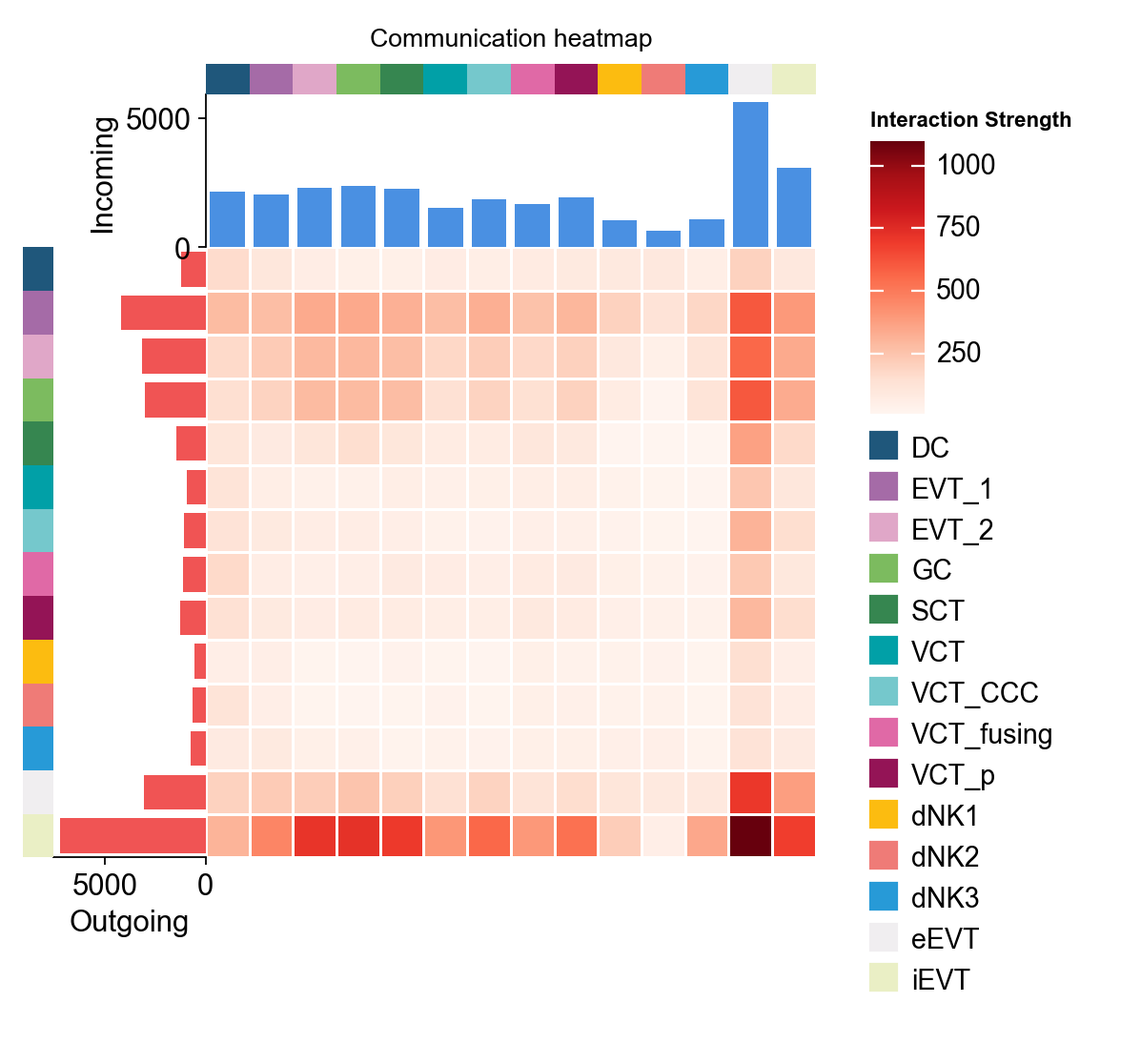
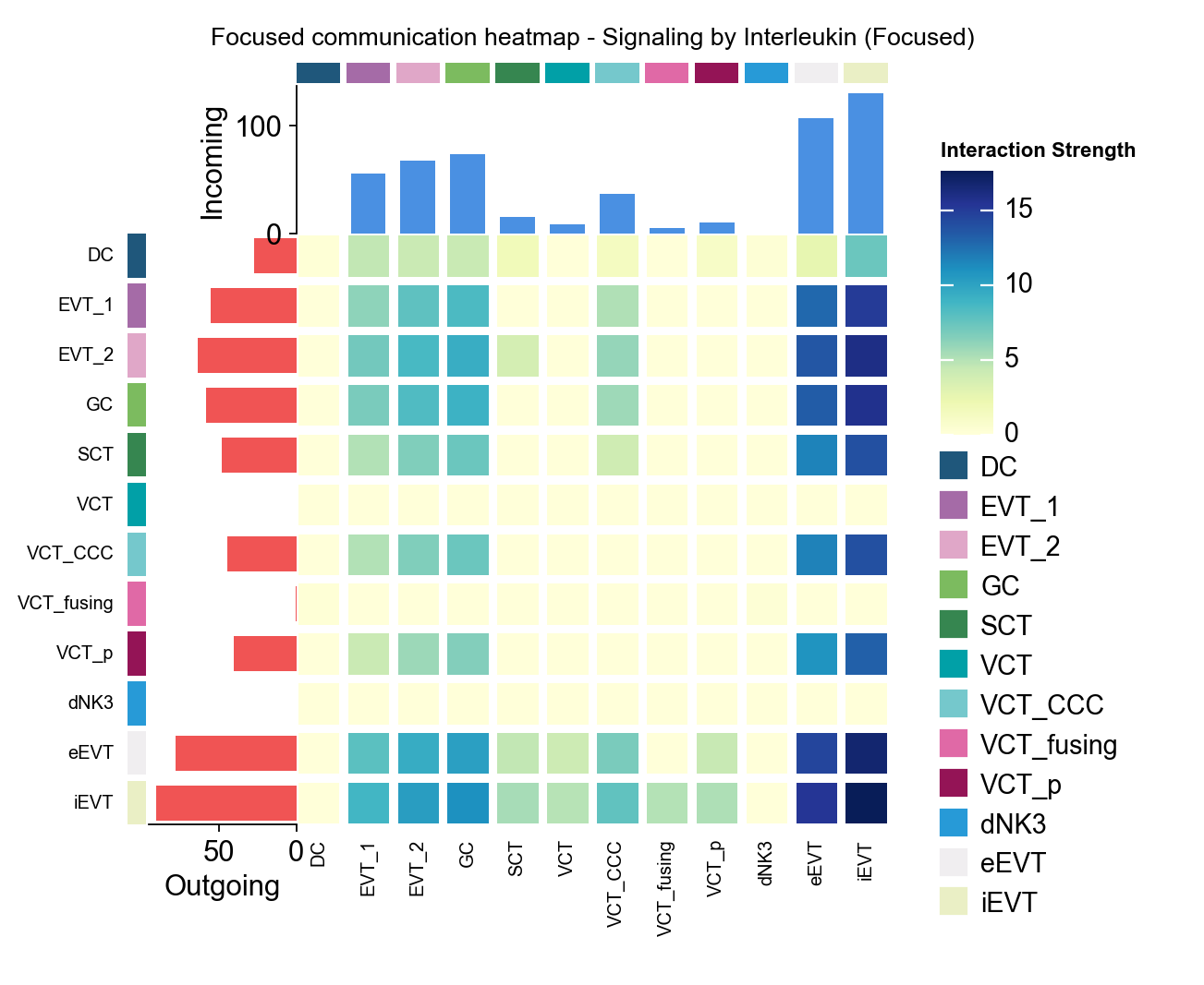
一、ov.pl.ccc_heatmap#
这部分以矩阵和分面图为主,重点回答:
哪些 pathway / interaction 在细胞群之间最强
sender / receiver 层面的矩阵结构是什么
role summary 是否偏 incoming / outgoing
1.1 aggregation heatmap 与 focused heatmap#
fig, ax = ov.pl.ccc_heatmap(
    adata,
    plot_type='heatmap',
    display_by='aggregation',
    cmap='Reds',
    show=False,
)
- Found 13 info columns and 196 cell type pairs
   - Found 121 pathway classifications
fig, ax = ov.pl.ccc_heatmap(
    adata_plot,
    plot_type='focused_heatmap',
    signaling=['Signaling by Interleukin'],
    min_interaction_threshold=0.1,
    cmap='YlGnBu',
    figsize=(7, 5),
    show=False,
    show_row_names=True,
    show_col_names=True,
)
- Found 13 info columns and 196 cell type pairs
   - Found 121 pathway classifications
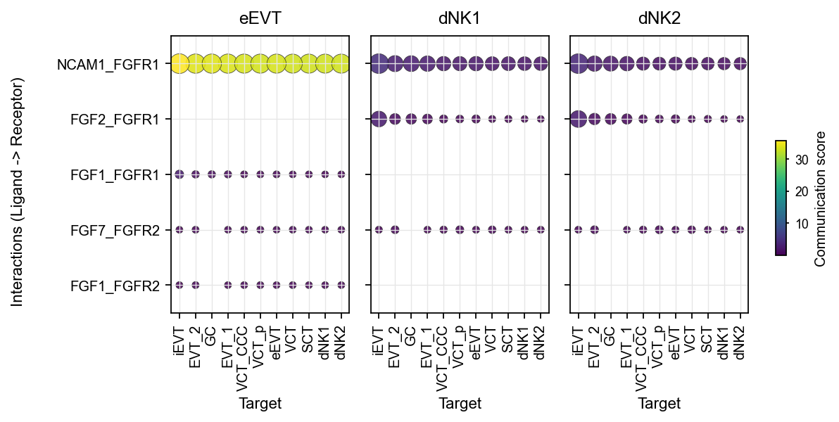
1.2 dot / pathway_bubble / role 类热图#
fig, ax = ov.pl.ccc_heatmap(
    adata_plot,
    plot_type='dot',
    sender_use=['eEVT', 'dNK1', 'dNK2'],
    display_by='interaction',
    signaling=[focus_pathway],
    top_n=5,
    cmap='viridis',
    figsize=(8, 3),
    show=False,
)
- Found 13 info columns and 196 cell type pairs
   - Found 121 pathway classifications
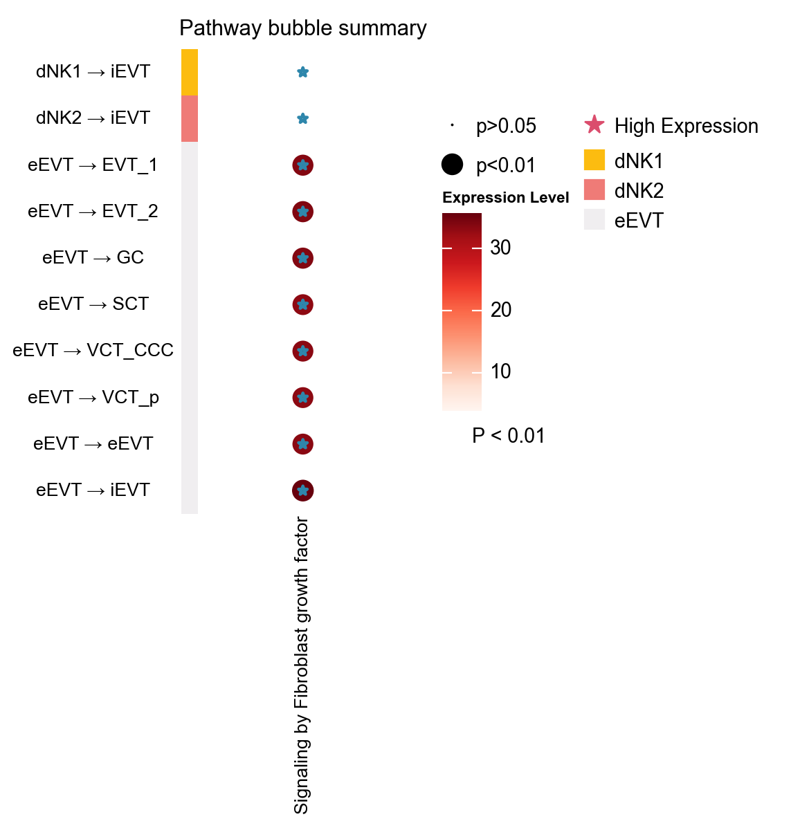
fig, ax = ov.pl.ccc_heatmap(
    adata_plot,
    plot_type='pathway_bubble',
    signaling=[focus_pathway],
    top_n=10,
    figsize=(3, 6),
    show=False,
)
- Found 13 info columns and 196 cell type pairs
   - Found 121 pathway classifications
⚠️  Warning: All p-values are identical. Adding slight jitter for better visualization.
⚠️  Warning: All p-values are identical after jittering. Using medium size.
📊 Visualization statistics:
   - Number of significant interactions: 10
   - Number of cell type pairs: 10
   - Signaling pathways: 1
   - Data scaling: None (raw expression values)
   - Color bars: sender
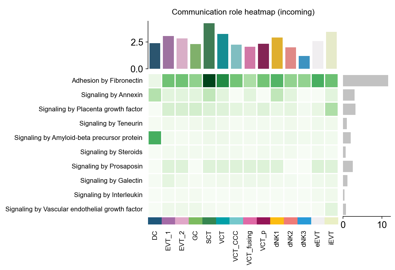
fig, ax = ov.pl.ccc_heatmap(
    adata_plot,
    plot_type='role_heatmap',
    pattern='incoming',
    cmap='Greens',
    top_n=10,
    figsize=(4, 3),
    show=False,
)
- Found 13 info columns and 196 cell type pairs
   - Found 121 pathway classifications
🔬 Calculating cell communication strength for 121 pathways...
   - Aggregation method: mean
   - Minimum expression threshold: 0.1
✅ Completed pathway communication strength calculation for 121 pathways
📊 Pathway significance analysis results:
   - Total pathways: 121
   - Significant pathways: 72
   - Strength threshold: 0.5
   - p-value threshold: 0.05

🏆 Top 10 pathways by total strength:
----------------------------------------------------------------------------------------------------
Pathway                        Total    Max     Mean    L-R  Active Sig  Rate   Status
----------------------------------------------------------------------------------------------------
Adhesion by Fibronectin        4488.87  145.91  22.90   12   196    52   0.27   ***
Signaling by Annexin           885.09   26.18   6.32    2    140    7    0.05   ***
Signaling by Placenta growth   829.15   21.65   5.06    4    164    59   0.36   ***
Signaling by Teneurin          734.99   10.64   4.15    12   177    43   0.24   ***
Signaling by Amyloid-beta pr   613.11   26.05   3.18    5    193    63   0.33   ***
Signaling by Steroids          504.07   38.99   3.17    10   159    10   0.06   ***
Signaling by Prosaposin        495.83   11.05   3.54    1    140    25   0.18   ***
Signaling by Galectin          446.87   11.45   2.39    4    187    42   0.22   ***
Signaling by Interleukin       436.29   15.95   2.41    14   181    60   0.33   ***
Signaling by Vascular endoth   410.57   10.17   2.32    12   177    57   0.32   ***
📊 Heatmap statistics:
   - Number of pathways: 10
   - Number of cell types: 14
   - Signal strength range: 0.000 - 22.650
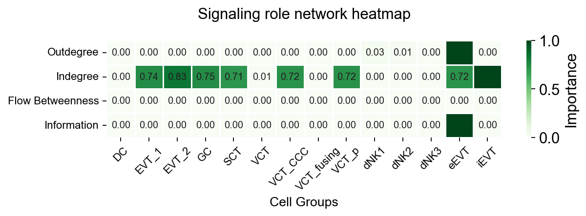
fig, ax = ov.pl.ccc_heatmap(
    adata_plot,
    plot_type='role_network',
    signaling=[focus_pathway],
    cmap='Greens',
    figsize=(8, 3),
    show=False,
)
- Found 13 info columns and 196 cell type pairs
   - Found 121 pathway classifications
✅ Network centrality calculation completed (CellChat-style Importance values)
   - Signaling pathways used: ['Signaling by Fibroblast growth factor']
   - Weight mode: Weighted
   - Calculated metrics: outdegree, indegree, flow_betweenness, information, overall
   - All centrality scores normalized to 0-1 range (Importance values)
📊 Signaling role analysis results (Importance values 0-1):
   - Dominant Sender: eEVT (Importance: 1.000)
   - Dominant Receiver: iEVT (Importance: 1.000)
   - Influencer: eEVT (Importance: 1.000)
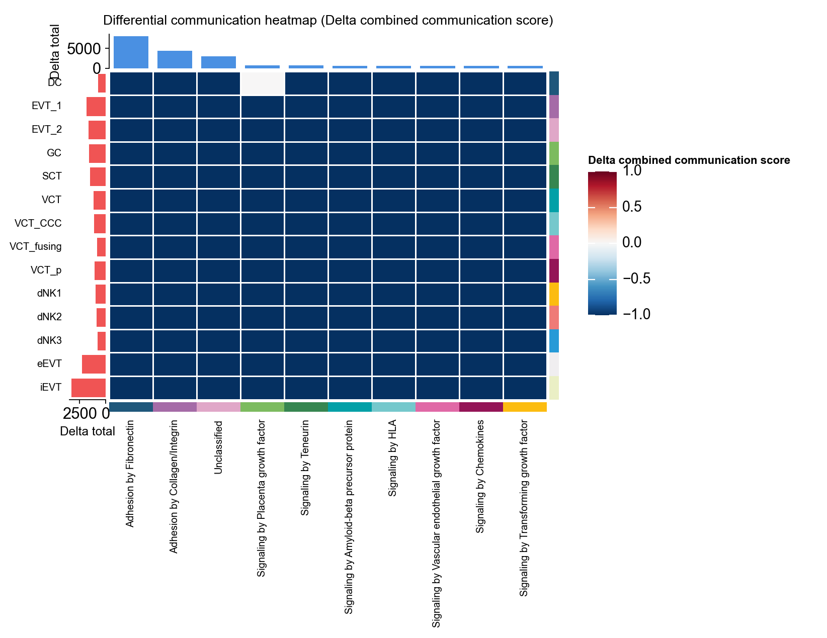
1.3 差异热图#
fig, ax = ov.pl.ccc_heatmap(
    comm_adata,
    comparison_adata=comparison_comm,
    plot_type='diff_heatmap',
    top_n=10,
    show=False,
    show_col_names=True,
    show_row_names=True,
)
二、ov.pl.ccc_network_plot#
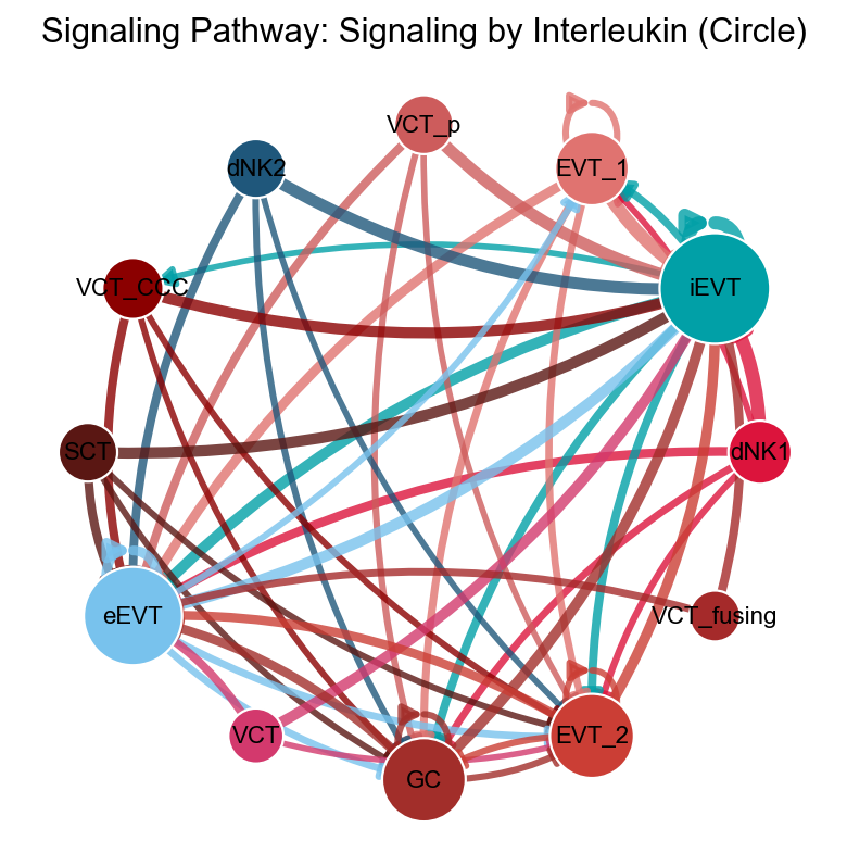
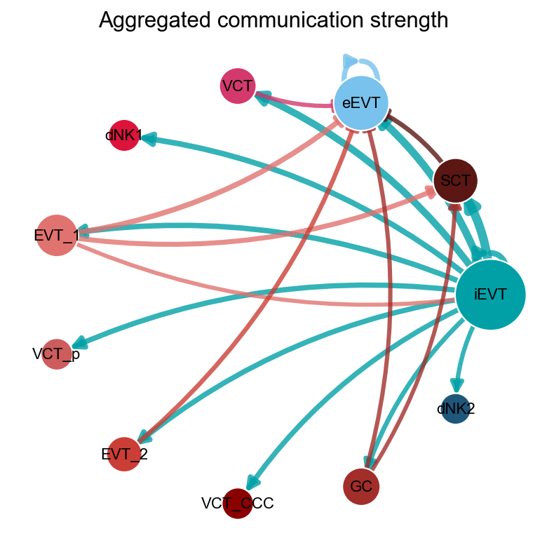
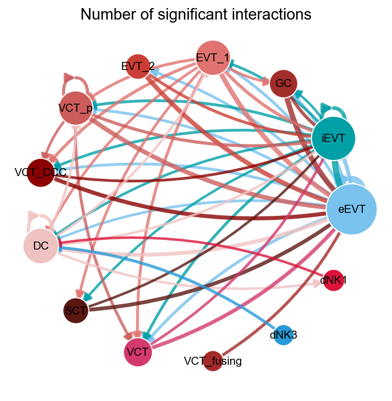
网络类视图适合从“总体结构”和“流向”角度理解通讯结果。
fig, ax = ov.pl.ccc_network_plot(
    adata_plot,
    plot_type='pathway',
    signaling=['Signaling by Interleukin'],
    palette=color_dict,
    top_n=50,
    figsize=(6, 6),
    show=False,
)
- Found 13 info columns and 196 cell type pairs
   - Found 121 pathway classifications
fig, ax = ov.pl.ccc_network_plot(
    adata_plot,
    plot_type='circle',
    palette=color_dict,
    title='Aggregated communication strength',
    figsize=(6, 6),
    show=False,
)
- Found 13 info columns and 196 cell type pairs
   - Found 121 pathway classifications
fig, ax = ov.pl.ccc_network_plot(
    adata_plot,
    plot_type='circle',
    value='count',
    palette=color_dict,
    top_n=50,
    title='Number of significant interactions',
    figsize=(6, 6),
    show=False,
)
- Found 13 info columns and 196 cell type pairs
   - Found 121 pathway classifications
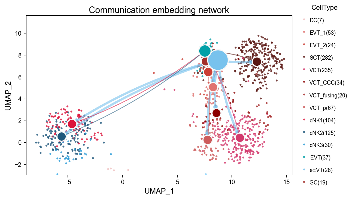
fig, ax = ov.pl.ccc_network_plot(
    comm_adata,
    plot_type='embedding_network',
    signaling=[focus_pathway],
    node_positions=node_positions,
    embedding_points=embedding_points,
    palette=color_dict,
    top_n=20,
    figsize=(7, 7),
    show=False,
)
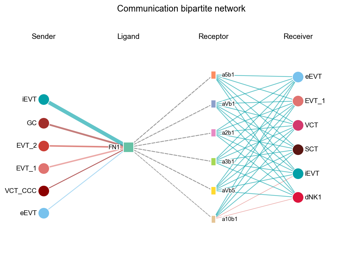
fig, ax = ov.pl.ccc_network_plot(
    adata,
    plot_type='bipartite',
    ligand=focus_ligand,
    palette=color_dict,
    top_n=6,
    figsize=(8, 6),
    show=False,
)
- Found 13 info columns and 196 cell type pairs
   - Found 121 pathway classifications
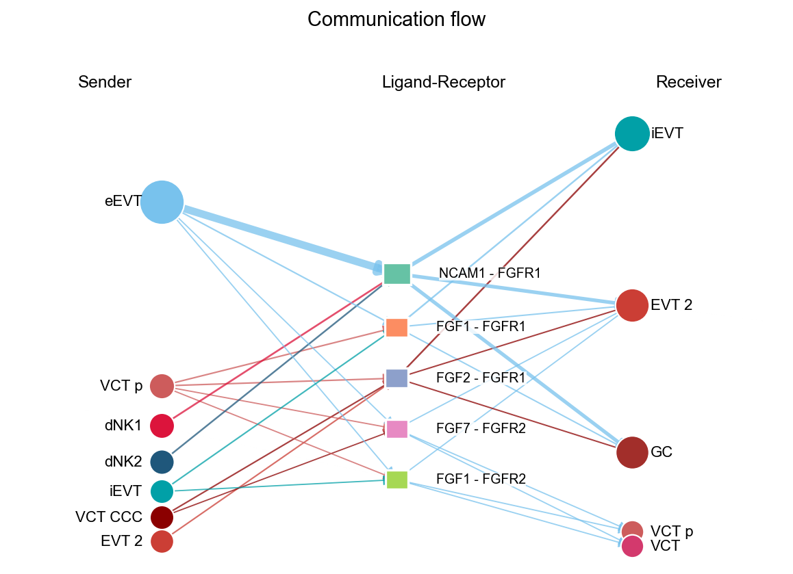
fig, ax = ov.pl.ccc_network_plot(
    comm_adata,
    plot_type='arrow',
    display_by='interaction',
    signaling=[focus_pathway],
    palette=color_dict,
    top_n=5,
    figsize=(8, 6),
    show=False,
)
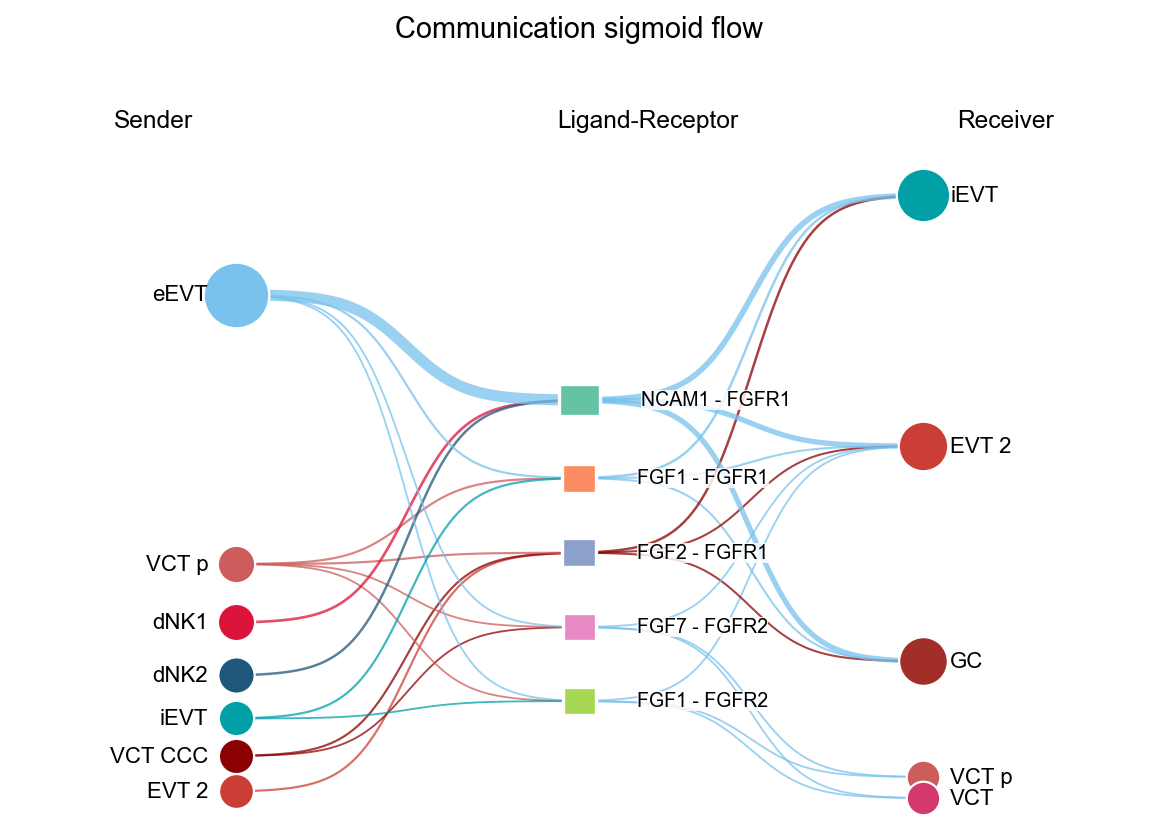
fig, ax = ov.pl.ccc_network_plot(
    comm_adata,
    plot_type='sigmoid',
    display_by='interaction',
    signaling=[focus_pathway],
    palette=color_dict,
    top_n=5,
    figsize=(8, 6),
    show=False,
)
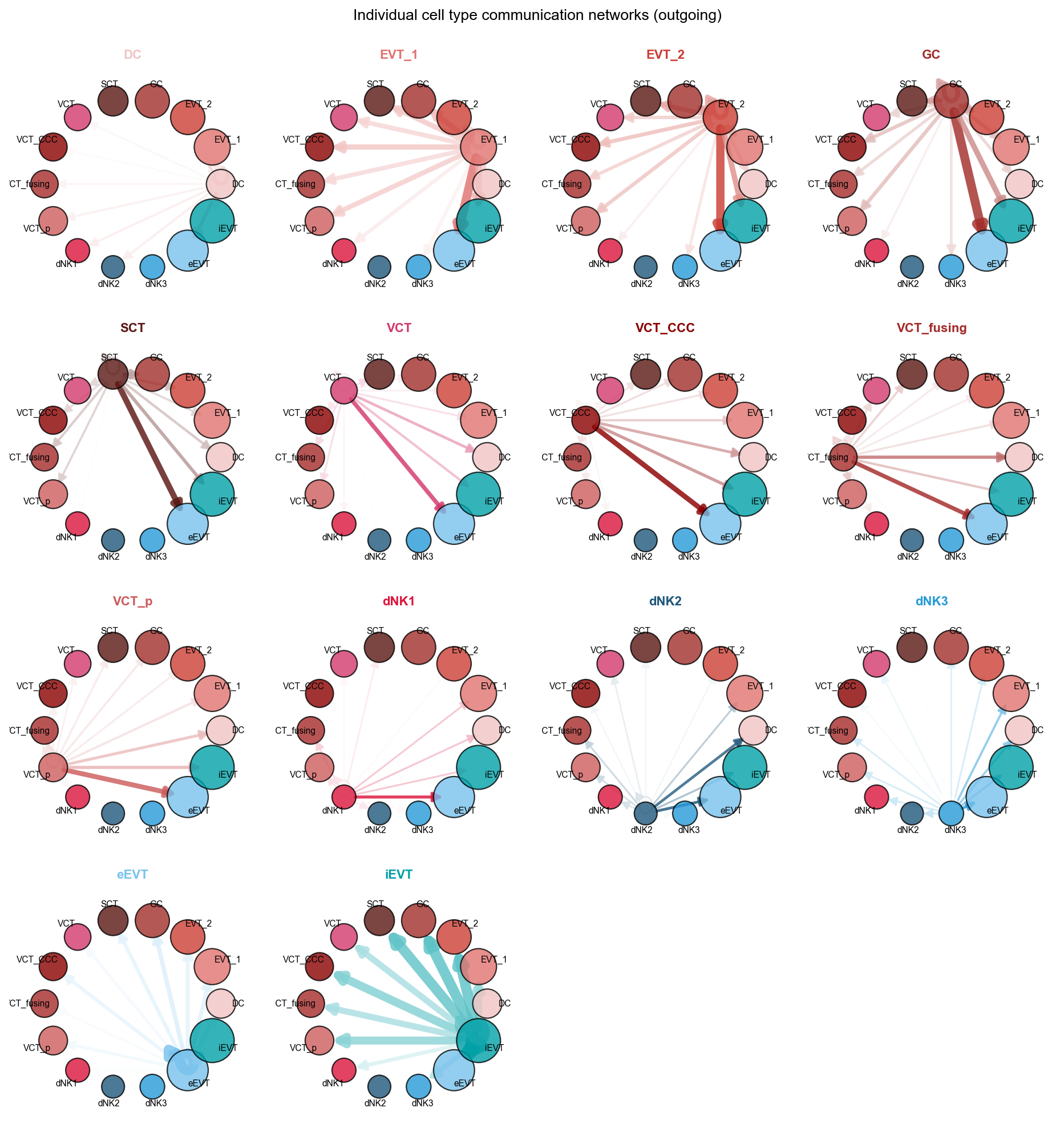
fig, ax = ov.pl.ccc_network_plot(
    comm_adata,
    plot_type='individual_outgoing',
    palette=color_dict,
    figsize=(12, 13),
    show=False,
)
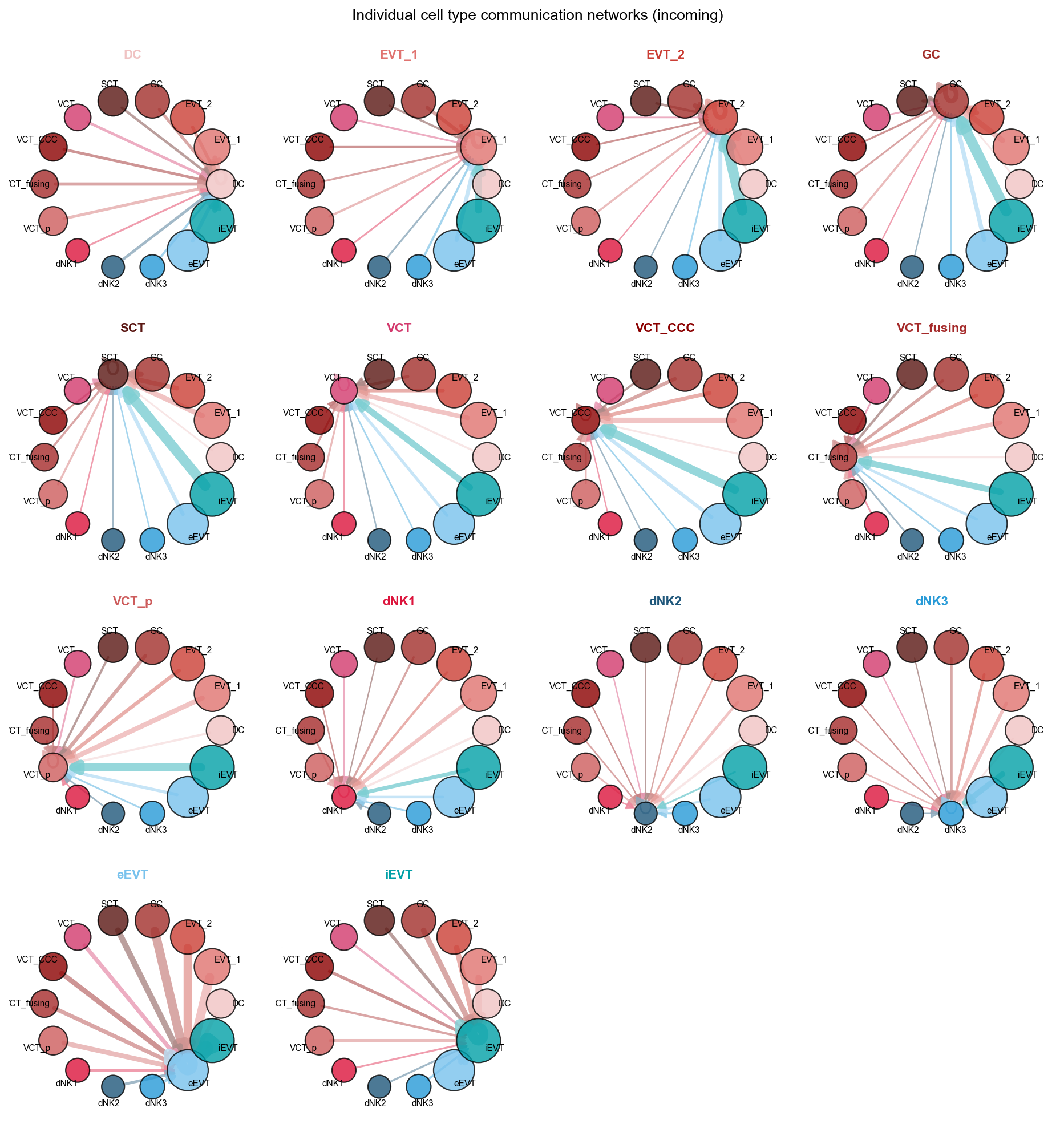
fig, ax = ov.pl.ccc_network_plot(
    comm_adata,
    plot_type='individual_incoming',
    palette=color_dict,
    figsize=(12, 13),
    show=False,
)
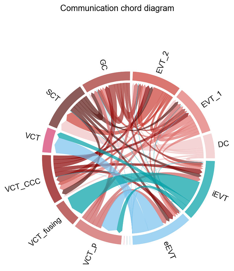
fig, ax = ov.pl.ccc_network_plot(
    comm_adata,
    plot_type='chord',
    signaling=['Signaling by Interleukin'],
    palette=color_dict,
    normalize_to_sender=True,
    figsize=(6, 6),
    show=False,
)
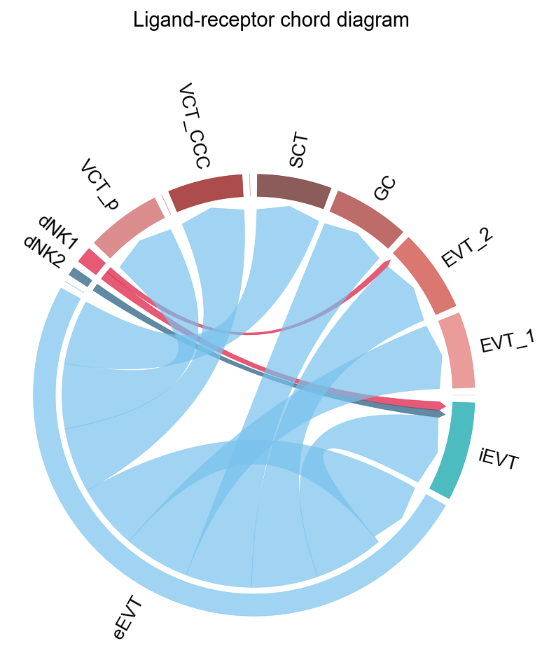
fig, ax = ov.pl.ccc_network_plot(
    comm_adata,
    plot_type='lr_chord',
    pair_lr_use=focus_pair_lr,
    palette=color_dict,
    figsize=(6, 6),
    show=False,
)
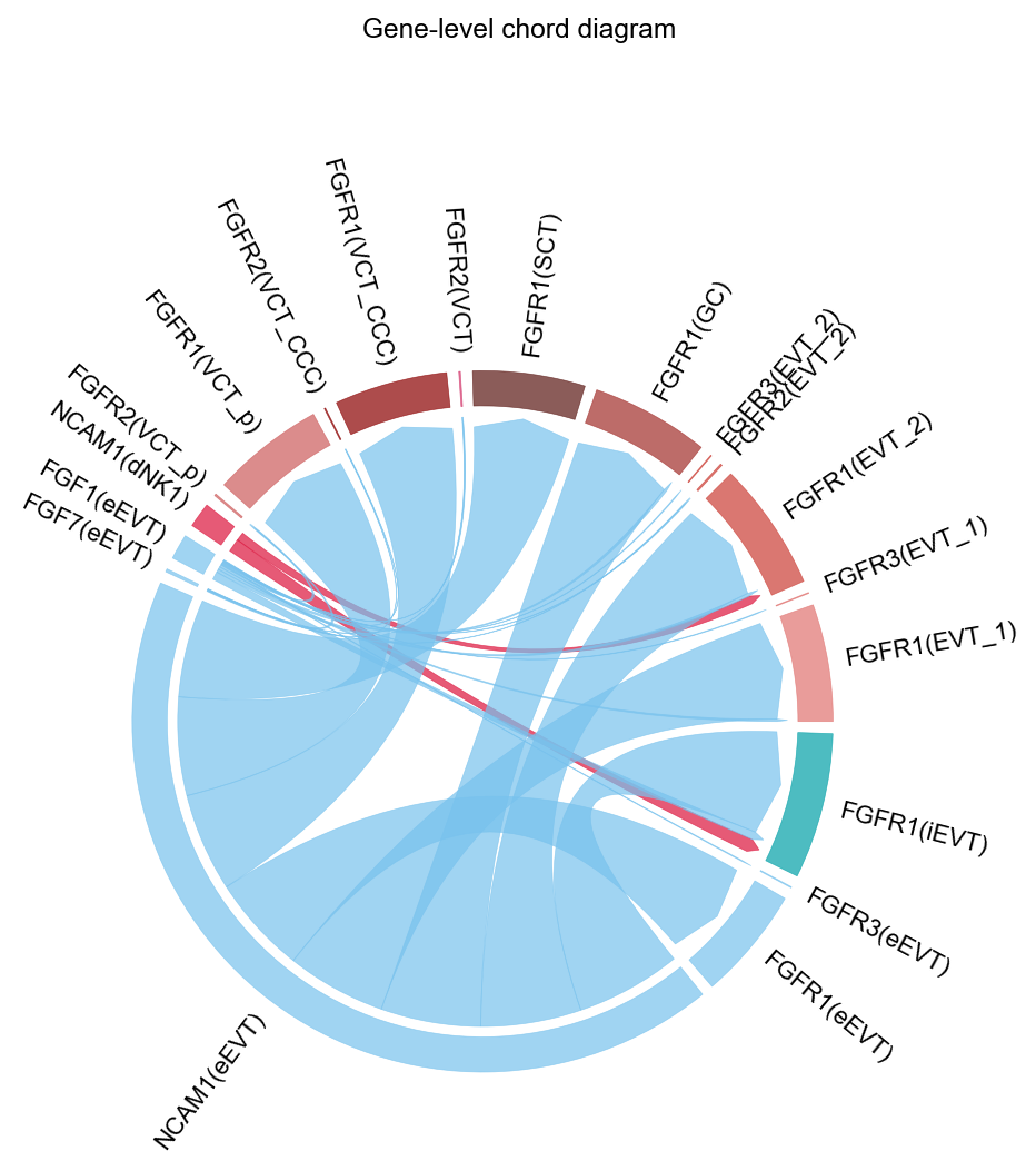
fig, ax = ov.pl.ccc_network_plot(
    comm_adata,
    plot_type='gene_chord',
    signaling=['Signaling by Fibroblast growth factor'],
    sender_use=['eEVT', 'dNK1'],
    palette=color_dict,
    figsize=(6, 7),
    show=False,
)
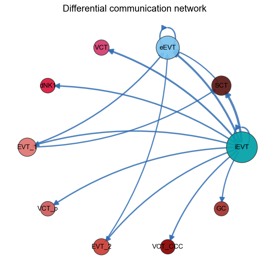
fig, ax = ov.pl.ccc_network_plot(
    comm_adata,
    comparison_adata=comparison_comm,
    plot_type='diff_network',
    palette=color_dict,
    top_n=15,
    show=False,
)
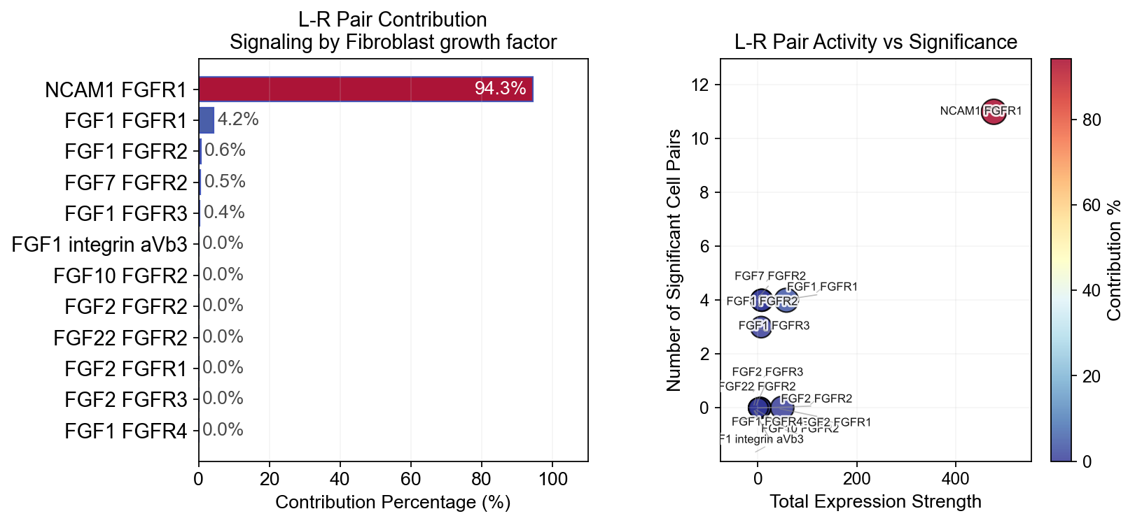
三、ov.pl.ccc_stat_plot#
统计总结图适合做排序、贡献分析和路径压缩解释。
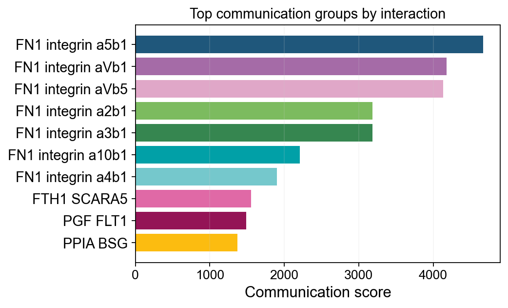
fig, ax = ov.pl.ccc_stat_plot(
    adata_plot,
    plot_type='bar',
    figsize=(6, 4),
    top_n=10,
    show=False,
)
- Found 13 info columns and 196 cell type pairs
   - Found 121 pathway classifications
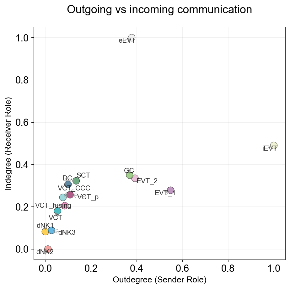
fig, ax = ov.pl.ccc_stat_plot(
    adata_plot,
    plot_type='scatter',
    figsize=(6, 6),
    show=False,
)
- Found 13 info columns and 196 cell type pairs
   - Found 121 pathway classifications
✅ Network centrality calculation completed (CellChat-style Importance values)
   - Signaling pathways used: All pathways
   - Weight mode: Weighted
   - Calculated metrics: outdegree, indegree, flow_betweenness, information, overall
   - All centrality scores normalized to 0-1 range (Importance values)
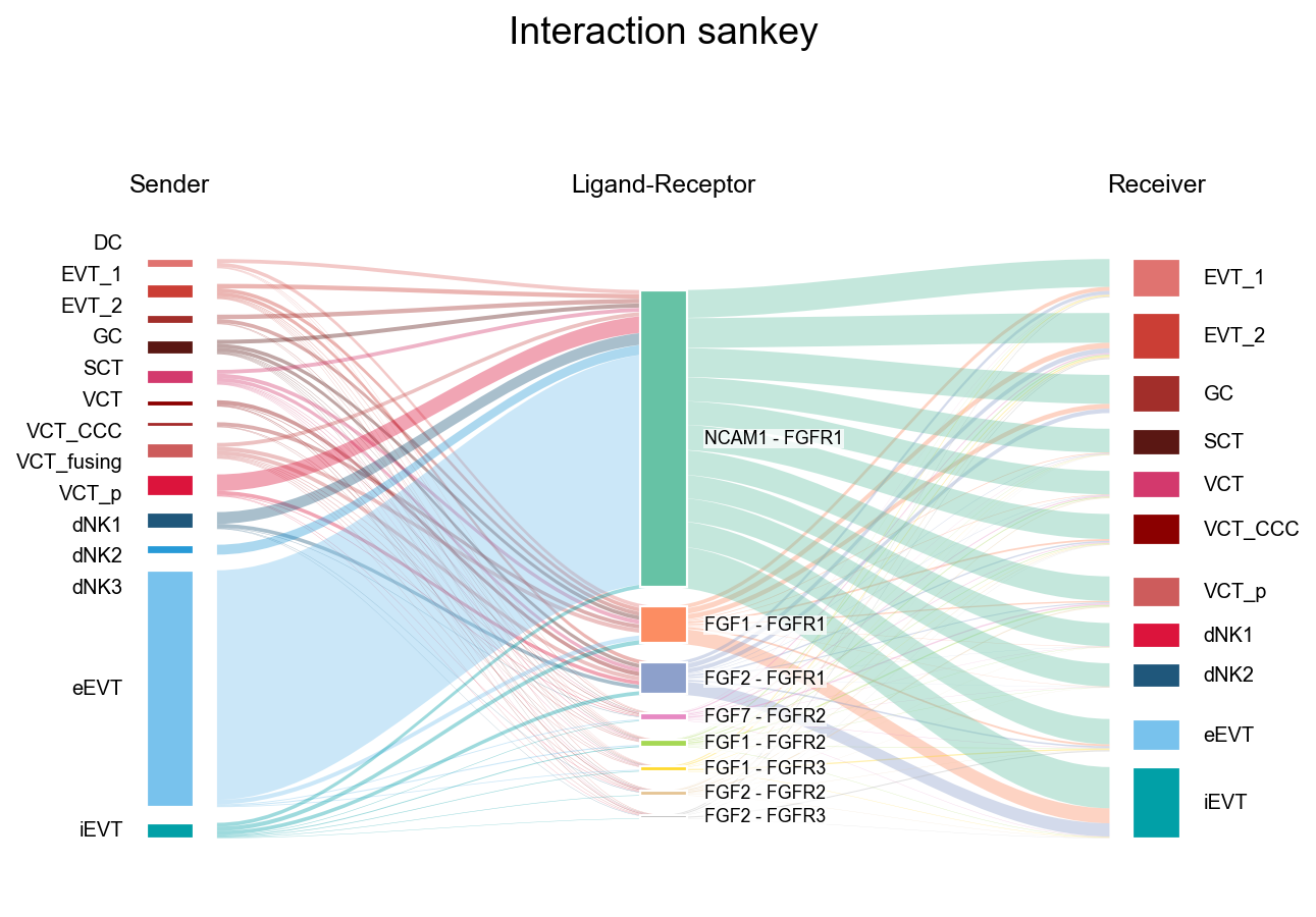
fig, ax = ov.pl.ccc_stat_plot(
    adata_plot,
    plot_type='sankey',
    display_by='interaction',
    signaling=[focus_pathway],
    palette=color_dict,
    top_n=8,
    figsize=(8, 6),
    show=False,
)
- Found 13 info columns and 196 cell type pairs
   - Found 121 pathway classifications
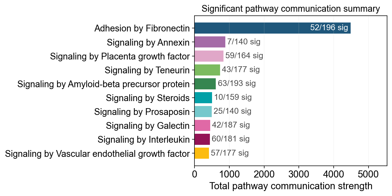
fig, ax = ov.pl.ccc_stat_plot(
    adata_plot,
    plot_type='pathway_summary',
    top_n=10,
    figsize=(5, 4),
    verbose=True,
    show=False,
)
- Found 13 info columns and 196 cell type pairs
   - Found 121 pathway classifications
🔬 Calculating cell communication strength for 121 pathways...
   - Aggregation method: mean
   - Minimum expression threshold: 0.1
✅ Completed pathway communication strength calculation for 121 pathways
📊 Pathway significance analysis results:
   - Total pathways: 121
   - Significant pathways: 72
   - Strength threshold: 0.5
   - p-value threshold: 0.05

🏆 Top 10 pathways by total strength:
----------------------------------------------------------------------------------------------------
Pathway                        Total    Max     Mean    L-R  Active Sig  Rate   Status
----------------------------------------------------------------------------------------------------
Adhesion by Fibronectin        4488.87  145.91  22.90   12   196    52   0.27   ***
Signaling by Annexin           885.09   26.18   6.32    2    140    7    0.05   ***
Signaling by Placenta growth   829.15   21.65   5.06    4    164    59   0.36   ***
Signaling by Teneurin          734.99   10.64   4.15    12   177    43   0.24   ***
Signaling by Amyloid-beta pr   613.11   26.05   3.18    5    193    63   0.33   ***
Signaling by Steroids          504.07   38.99   3.17    10   159    10   0.06   ***
Signaling by Prosaposin        495.83   11.05   3.54    1    140    25   0.18   ***
Signaling by Galectin          446.87   11.45   2.39    4    187    42   0.22   ***
Signaling by Interleukin       436.29   15.95   2.41    14   181    60   0.33   ***
Signaling by Vascular endoth   410.57   10.17   2.32    12   177    57   0.32   ***
fig, ax = ov.pl.ccc_stat_plot(
    adata_plot,
    plot_type='lr_contribution',
    signaling=['Signaling by Fibroblast growth factor'],
    figsize=(10, 5),
    show=False,
)
- Found 13 info columns and 196 cell type pairs
   - Found 121 pathway classifications