单细胞差异表达分析#
差异表达(DE)分析用于识别在不同细胞类型、条件或状态之间表达变化的基因。在单细胞数据的背景下,这涉及在细胞簇或细胞类型之间进行比较。本教程演示了如何在OmicVerse中进行全面的差异表达分析。
# 导入库
import omicverse as ov
import scanpy as sc
🔬 Starting plot initialization...
🧬 Detecting GPU devices…
✅ Apple Silicon MPS detected
    • [MPS] Apple Silicon GPU - Metal Performance Shaders available
✅ plot_set complete.
准备数据#
首先,我们加载并准备数据进行差异表达分析。
adata = pt.dt.haber_2017_regions()adata
AnnData object with n_obs × n_vars = 9842 × 15215
    obs: 'batch', 'barcode', 'condition', 'cell_label'
差异表达方法#
OmicVerse支持多种用于单细胞差异表达的方法。
# 加载示例数据
adata = ov.datasets.pbmc3k()
data = ov.pp.preprocess(adata)
AnnData object with n_obs × n_vars = 5010 × 15215
    obs: 'batch', 'barcode', 'condition', 'cell_label'
adata.obs["condition"].unique()
['Control', 'Salmonella']
Categories (2, object): ['Control', 'Salmonella']
Wilcoxon检验#
Wilcoxon秩和检验是用于识别差异表达基因的非参数检验。
deg_obj=ov.single.DEG( adata, condition='condition', ctrl_group='Control', test_group='Salmonella', method='wilcoxon',)deg_obj.run( celltype_key='cell_label', celltype_group=['TA'],)
✅ Differential expression analysis initialized
📊 DEG analysis using wilcoxon method
📊 Condition: condition, Control group: Control, Test group: Salmonella
📊 Celltype key: cell_label, Celltype group: ['TA']
Total cells: 533 will be used for DEG analysis
normalizing counts per cell
    finished (0:00:00)
ranking genes
    finished: added to `.uns['rank_genes_groups']`
    'names', sorted np.recarray to be indexed by group ids
    'scores', sorted np.recarray to be indexed by group ids
    'logfoldchanges', sorted np.recarray to be indexed by group ids
    'pvals', sorted np.recarray to be indexed by group ids
    'pvals_adj', sorted np.recarray to be indexed by group ids (0:00:00)
✅ wilcoxon DEG analysis completed
res_wilcoxon=deg_obj.get_results()res_wilcoxon.head()
| log2FC | pvalue | padj | qvalue | size | sig | -log(pvalue) | -log(qvalue) | |
|---|---|---|---|---|---|---|---|---|
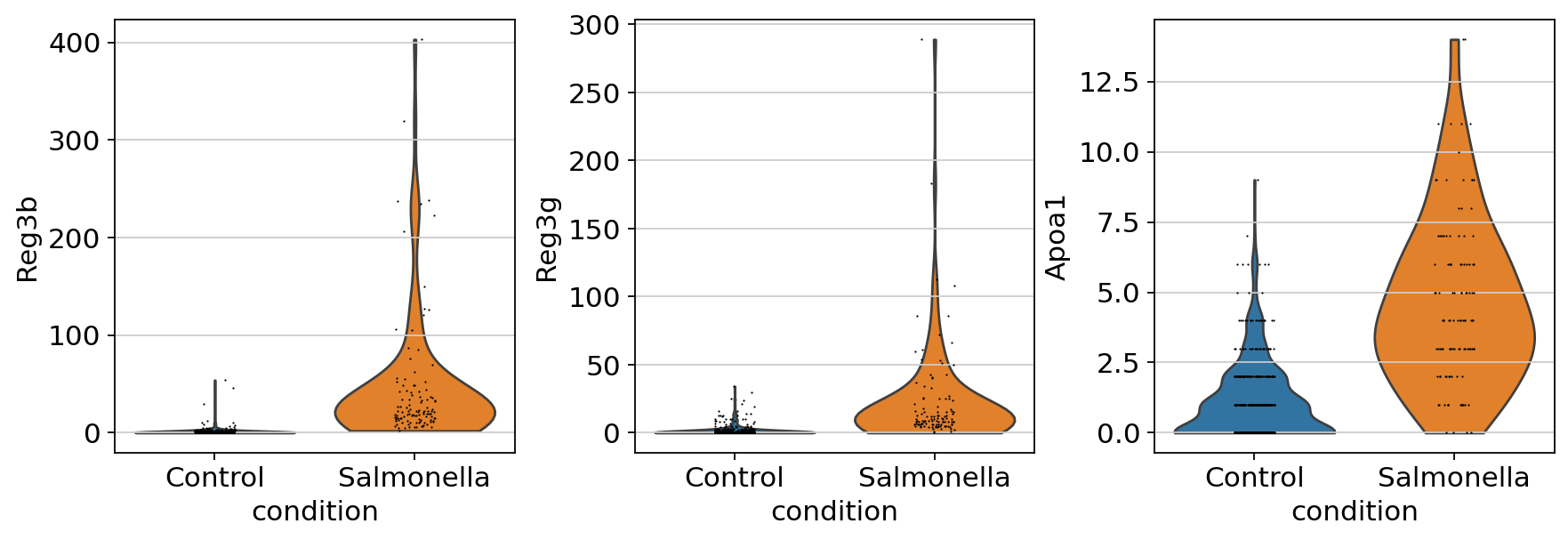
| Reg3b | 5.958403 | 2.899264e-58 | 4.411230e-54 | 4.411230e-54 | 0.595840 | sig | 57.537712 | 53.355440 |
| Reg3g | 4.425004 | 1.576382e-51 | 1.199233e-47 | 1.199233e-47 | 0.442500 | sig | 50.802339 | 46.921097 |
| Apoa1 | 2.589844 | 2.025723e-40 | 1.027379e-36 | 1.027379e-36 | 0.258984 | sig | 39.693420 | 35.988269 |
| Guca2b | 2.380329 | 1.732794e-21 | 5.272893e-18 | 5.272893e-18 | 0.238033 | sig | 20.761253 | 17.277951 |
| Zg16 | 2.077089 | 2.553716e-21 | 6.475798e-18 | 6.475798e-18 | 0.207709 | sig | 20.592827 | 17.188707 |
t检验和其他参数检验#
虽然Wilcoxon检验很常见,但其他参数检验也可用。
celltypes_li=['TA']sc.pl.violin( adata[adata.obs['cell_label'].isin(celltypes_li)], keys=['Reg3b','Reg3g','Apoa1'], groupby='condition')
多重检验校正#
在进行多个假设检验时,需要校正多重检验。
deg_obj=ov.single.DEG( adata, condition='condition', ctrl_group='Control', test_group='Salmonella', method='memento-de',)deg_obj.run( celltype_key='cell_label', celltype_group=['TA'], capture_rate=0.07, num_cpus=12, num_boot=5000)
✅ Differential expression analysis initialized
📊 DEG analysis using memento-de method
📊 Condition: condition, Control group: Control, Test group: Salmonella
📊 Celltype key: cell_label, Celltype group: ['TA']
Total cells: 533 will be used for DEG analysis
✅ memento-de DEG analysis completed
res_memento=deg_obj.get_results()res_memento.query('dv_coef > 1 & de_coef > 0').sort_values('dv_pval').head(5)
| gene | tx | de_coef | de_se | de_pval | dv_coef | dv_se | dv_pval | |
|---|---|---|---|---|---|---|---|---|
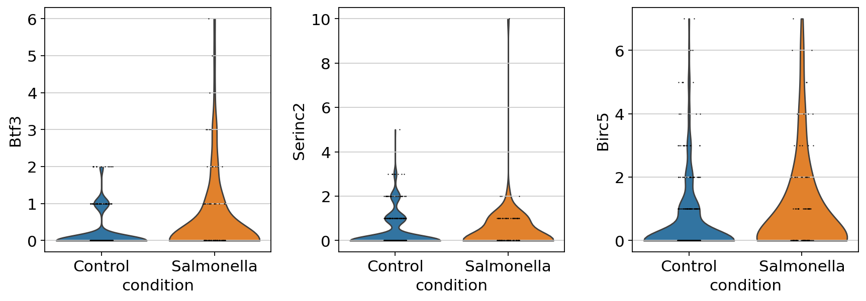
| 443 | Btf3 | stim | 0.838806 | 0.230108 | 0.000213 | 2.940342 | 0.580788 | 4.519054e-07 |
| 397 | Birc5 | stim | 0.631178 | 0.185273 | 0.000661 | 1.198823 | 0.313596 | 8.280704e-05 |
| 3421 | Serinc2 | stim | 0.030935 | 0.238055 | 0.826321 | 2.288608 | 0.511458 | 1.560657e-04 |
| 917 | Dcaf8 | stim | 0.037631 | 0.316794 | 0.846642 | 1.833301 | 0.500972 | 2.687823e-04 |
| 536 | Ccnb2 | stim | 0.132247 | 0.234056 | 0.565606 | 1.126923 | 0.323989 | 3.477457e-04 |
celltypes_li=['TA']sc.pl.violin( adata[adata.obs['cell_label'].isin(celltypes_li)], keys=['Btf3','Serinc2','Birc5'], groupby='condition')
火山图#
火山图是可视化差异表达结果的标准方法。
dct_obj=ov.single.DCT( adata, condition='condition', ctrl_group='Control', test_group='Salmonella', cell_type_key='cell_label', method='sccoda', sample_key='batch',)
• Automatic reference selection! Reference cell type set to Endocrine
热图#
热图用于可视化多个基因和细胞之间的表达模式。
# 基因表达热图
top_genes = de_results.loc[de_results['pvalue'] < 0.05].head(20).index
sc.pl.heatmap(adata, var_names=top_genes, groupby='leiden')
res=dct_obj.get_results()res.head()
| Final Parameter | HDI 3% | HDI 97% | SD | Inclusion probability | Expected Sample | log2-fold change | ||
|---|---|---|---|---|---|---|---|---|
| Covariate | Cell Type | |||||||
| conditionT.Salmonella | Endocrine | 0.000000 | 0.000 | 0.000 | 0.000 | 0.0000 | 25.782816 | -0.495162 |
| Enterocyte | 1.367619 | 0.864 | 1.886 | 0.262 | 1.0000 | 325.488661 | 1.477896 | |
| Enterocyte.Progenitor | 0.000000 | -0.393 | 0.647 | 0.163 | 0.3072 | 100.454836 | -0.495162 | |
| Goblet | 0.000000 | -0.228 | 1.037 | 0.298 | 0.4688 | 43.541227 | -0.495162 | |
| Stem | 0.000000 | -0.750 | 0.251 | 0.199 | 0.3560 | 120.266274 | -0.495162 |
通路富集分析#
识别差异表达基因后,我们可以进行通路富集分析。
dct_obj.model.set_fdr(dct_obj.sccoda_data, modality_key="coda", est_fdr=0.6)res=dct_obj.get_results()res.sort_values('Final Parameter',ascending=False).head()
| Final Parameter | HDI 3% | HDI 97% | SD | Inclusion probability | Expected Sample | log2-fold change | ||
|---|---|---|---|---|---|---|---|---|
| Covariate | Cell Type | |||||||
| conditionT.Salmonella | Enterocyte | 1.367619 | 0.864 | 1.886 | 0.262 | 1.0000 | 327.583710 | 1.487152 |
| Goblet | 0.353104 | -0.228 | 1.037 | 0.298 | 0.4688 | 62.378974 | 0.023516 | |
| Enterocyte.Progenitor | 0.115878 | -0.393 | 0.647 | 0.163 | 0.3072 | 113.522620 | -0.318729 | |
| TA.Early | 0.008501 | -0.408 | 0.486 | 0.121 | 0.2748 | 142.968607 | -0.473642 | |
| Endocrine | 0.000000 | 0.000 | 0.000 | 0.000 | 0.0000 | 25.948771 | -0.485906 |
# GSEA富集分析
gsea_results = ov.single.gsea(adata, gene_sets='kegg', groupby='leiden')
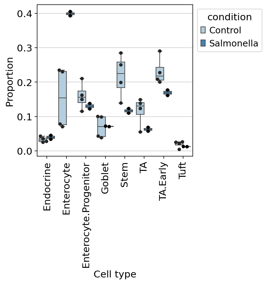
dct_obj.model.summary( dct_obj.sccoda_data, modality_key="coda")
                                          Compositional Analysis summary
┌──────────────────────────────────────────────┬──────────────────────────────────────────────────────────────────┐
│ Name                                         │ Value                                                            │
├──────────────────────────────────────────────┼──────────────────────────────────────────────────────────────────┤
│ Data                                         │ Data: 6 samples, 8 cell types                                    │
│ Reference cell type                          │ Endocrine                                                        │
│ Formula                                      │ condition                                                        │
└──────────────────────────────────────────────┴──────────────────────────────────────────────────────────────────┘
┌─────────────────────────────────────────────────────────────────────────────────────────────────────────────────┐
│ Intercepts                                                                                                      │
├─────────────────────────────────────────────────────────────────────────────────────────────────────────────────┤
│                        Final Parameter  Expected Sample                                                         │
│ Cell Type                                                                                                       │
│ Endocrine                  1.183            36.340                                                              │
│ Enterocyte                 2.351           116.854                                                              │
│ Enterocyte.Progenitor      2.543           141.589                                                              │
│ Goblet                     1.707            61.370                                                              │
│ Stem                       2.723           169.513                                                              │
│ TA                         2.126            93.310                                                              │
│ TA.Early                   2.881           198.528                                                              │
│ Tuft                       0.452            17.495                                                              │
└─────────────────────────────────────────────────────────────────────────────────────────────────────────────────┘
┌─────────────────────────────────────────────────────────────────────────────────────────────────────────────────┐
│ Effects                                                                                                         │
├─────────────────────────────────────────────────────────────────────────────────────────────────────────────────┤
│                                              Final Parameter  Expected Sample  log2-fold change                 │
│ Covariate             Cell Type                                                                                 │
│ conditionT.Salmonella Endocrine                   0.000           25.949            -0.486                      │
│                       Enterocyte                  1.368          327.584             1.487                      │
│                       Enterocyte.Progenitor       0.116          113.523            -0.319                      │
│                       Goblet                      0.353           62.379             0.024                      │
│                       Stem                       -0.229           96.260            -0.816                      │
│                       TA                         -0.212           53.916            -0.791                      │
│                       TA.Early                    0.009          142.969            -0.474                      │
│                       Tuft                       -0.006           12.421            -0.494                      │
└─────────────────────────────────────────────────────────────────────────────────────────────────────────────────┘
跨数据集的差异表达#
在多个数据集中识别一致的差异表达基因。
结果解释#
正确解释差异表达结果对下游分析至关重要。
ov.settings.cpu_gpu_mixed_init()
CPU-GPU mixed mode activated
adata=ov.pp.preprocess(adata,mode='shiftlog|pearson',n_HVGs=2000, target_sum=50*1e4)adata.raw = adataadata = adata[:, adata.var.highly_variable_features]ov.single.batch_correction(adata,batch_key='batch', methods='harmony',n_pcs=50)ov.pp.neighbors(adata, n_neighbors=15, n_pcs=50, use_rep='X_harmony')ov.pp.umap(adata)
Begin robust gene identification
After filtration, 15215/15215 genes are kept.     Among 15215 genes, 15215 genes are robust.
End of robust gene identification.
Begin size normalization: shiftlog and HVGs selection pearson
normalizing counts per cell. The following highly-expressed genes are not considered during normalization factor computation:
['Defa24', 'Fabp6', 'Gcg', 'Gip', 'Nts', 'Reg3b', 'Reg4', 'Sct', 'Spink4', 'Sst', 'Tff3', 'Zg16']
    finished (0:00:00)
extracting highly variable genes
--> added
    'highly_variable', boolean vector (adata.var)
    'highly_variable_rank', float vector (adata.var)
    'highly_variable_nbatches', int vector (adata.var)
    'highly_variable_intersection', boolean vector (adata.var)
    'means', float vector (adata.var)
    'variances', float vector (adata.var)
    'residual_variances', float vector (adata.var)
Time to analyze data in cpu: 7.434457540512085 seconds.
End of size normalization: shiftlog and HVGs selection pearson
...Begin using harmony to correct batch effect
🚀 Using GPU to calculate PCA...
📊 [GPU 0] ------------------------------ 5/12288 MiB (0.0%)
computing PCA🔍
    with n_comps=50
    finished✅ (0:00:01)
🖥️ Using Scanpy CPU to calculate neighbors...
computing neighbors
    finished: added to `.uns['neighbors']`
    `.obsp['distances']`, distances for each pair of neighbors
    `.obsp['connectivities']`, weighted adjacency matrix (0:00:02)
🔍 [2025-05-24 03:28:52] Running UMAP in 'cpu-gpu-mixed' mode...
🚀 Using torch GPU to calculate UMAP...
📊 [GPU 0] ------------------------------ 5/12288 MiB (0.0%)
computing UMAP🚀
    finished ✅: added
    'X_umap', UMAP coordinates (adata.obsm)
    'umap', UMAP parameters (adata.uns) (0:00:05)
✅ UMAP completed successfully.
adata=ov.read('data/milo_test.h5ad')
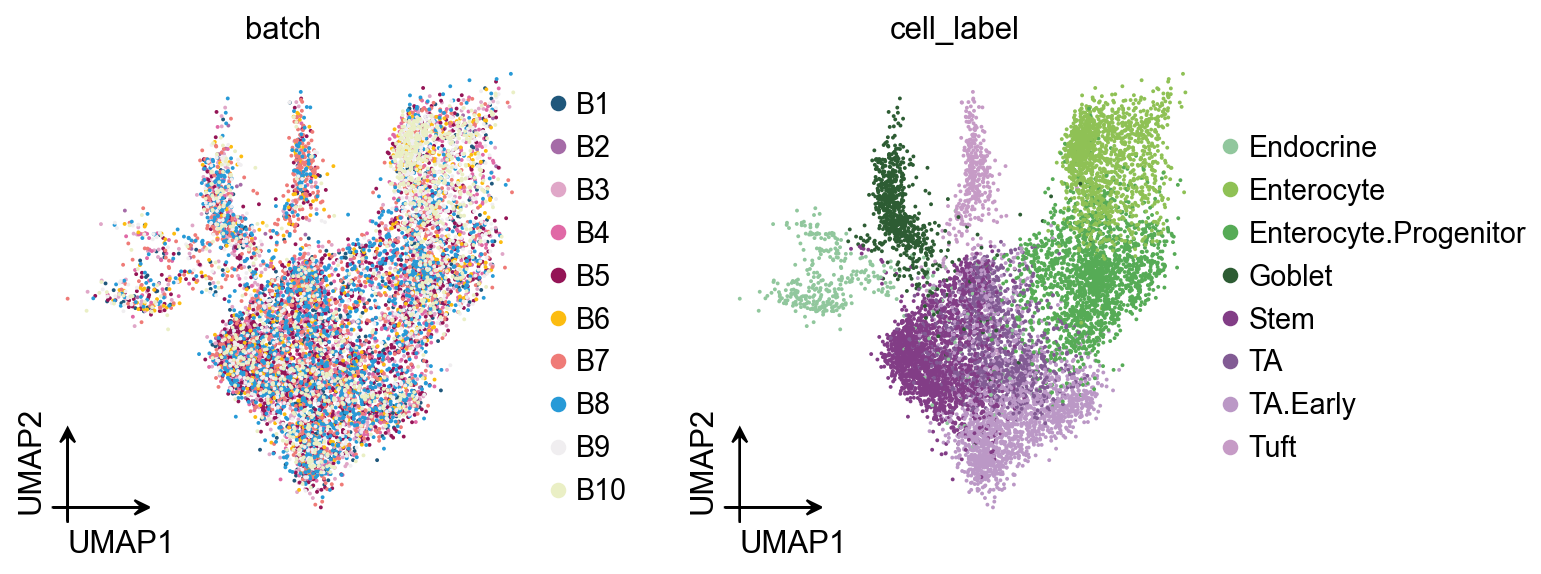
ov.pl.umap( adata, color=['batch','cell_label'],)
X_umap converted to UMAP to visualize and saved to adata.obsm['UMAP']
if you want to use X_umap, please set convert=False
处理混杂因素#
在某些分析中,需要考虑和调整混杂因素。
dct_obj=ov.single.DCT( adata, condition='condition', ctrl_group='Control', test_group='Salmonella', cell_type_key='cell_label', method='milopy', sample_key='batch', use_rep='X_harmony')
✅ Differential cell type abundance analysis initialized
📊 DCT analysis using milopy method
📊 Condition: condition, Control group: Control, Test group: Salmonella
computing neighbors
    finished: added to `.uns['neighbors']`
    `.obsp['distances']`, distances for each pair of neighbors
    `.obsp['connectivities']`, weighted adjacency matrix (0:00:21)
dct_obj.run()
✅ milopy DCT analysis completed
整合多个检验#
虽然我们展示了各个方法,但整合来自多个检验的结果通常会产生更可靠的结果。
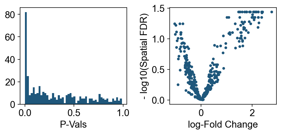
import matplotlib.pyplot as pltold_figsize = plt.rcParams["figure.figsize"]plt.rcParams["figure.figsize"] = [6, 3]plt.subplot(1, 2, 1)plt.hist(dct_obj.mdata["milo"].var.PValue, bins=50)plt.xlabel("P-Vals")plt.subplot(1, 2, 2)plt.plot(dct_obj.mdata["milo"].var.logFC, -ov.np.log10(dct_obj.mdata["milo"].var.SpatialFDR), ".")plt.xlabel("log-Fold Change")plt.ylabel("- log10(Spatial FDR)")plt.tight_layout()plt.rcParams["figure.figsize"] = old_figsize
常见陷阱#
在进行差异表达分析时需要避免几个常见问题。
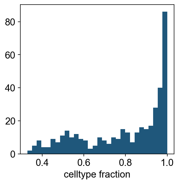
plt.hist(dct_obj.mdata["milo"].var["nhood_annotation_frac"], bins=30)plt.xlabel("celltype fraction")
Text(0.5, 0, 'celltype fraction')
res=dct_obj.get_results(mix_threshold=0.6)res.head()
| index_cell | kth_distance | logFC | lfcSE | logCPM | stat | PValue | FDR | adj_pvalue | SpatialFDR | Nhood_size | nhood_annotation | nhood_annotation_frac | |
|---|---|---|---|---|---|---|---|---|---|---|---|---|---|
| 0 | B1_AAACGCACTGTCCC_Control_Stem | 9.152347 | -0.583312 | 0.051568 | 11.412487 | 3.713398 | 0.080774 | 0.258990 | 0.258990 | 0.256133 | 399.0 | Mixed | 0.578947 |
| 1 | B1_AATAAGCTAGAGAT_Control_Enterocyte.Progenitor | 9.476911 | -0.809424 | 0.056194 | 11.429808 | 8.896907 | 0.012736 | 0.079455 | 0.079455 | 0.079067 | 408.0 | Mixed | 0.524510 |
| 2 | B1_ACGCTGCTCTCTTA_Control_Enterocyte.Progenitor | 9.004735 | 1.512198 | 0.017016 | 10.817280 | 12.689494 | 0.004606 | 0.045980 | 0.045980 | 0.044634 | 228.0 | Mixed | 0.557018 |
| 3 | B1_ACGGAACTGTTAGC_Control_Enterocyte.Progenitor | 9.966439 | 0.673496 | 0.032412 | 10.452936 | 2.316397 | 0.156838 | 0.362072 | 0.362072 | 0.350619 | 181.0 | Mixed | 0.563536 |
| 4 | B1_ACTTCTGATCGTTT_Control_TA.Early | 9.194638 | 0.202095 | 0.035912 | 11.222971 | 0.404716 | 0.537956 | 0.714916 | 0.714916 | 0.705203 | 339.0 | TA.Early | 0.820059 |
进一步阅读#
有许多资源可了解更多关于单细胞差异表达分析的信息。
# 保存差异表达结果
de_results.to_csv('deg_results.csv')
# 创建总结性绘图
fig, axes = plt.subplots(2, 2, figsize=(12, 10))
# 添加各种可视化
plt.tight_layout()
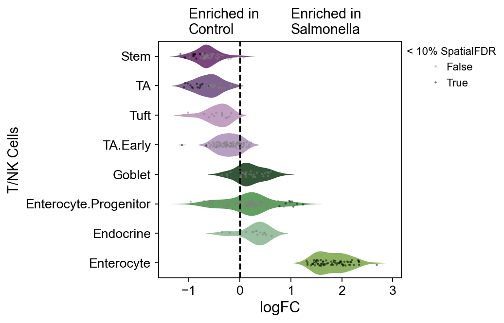
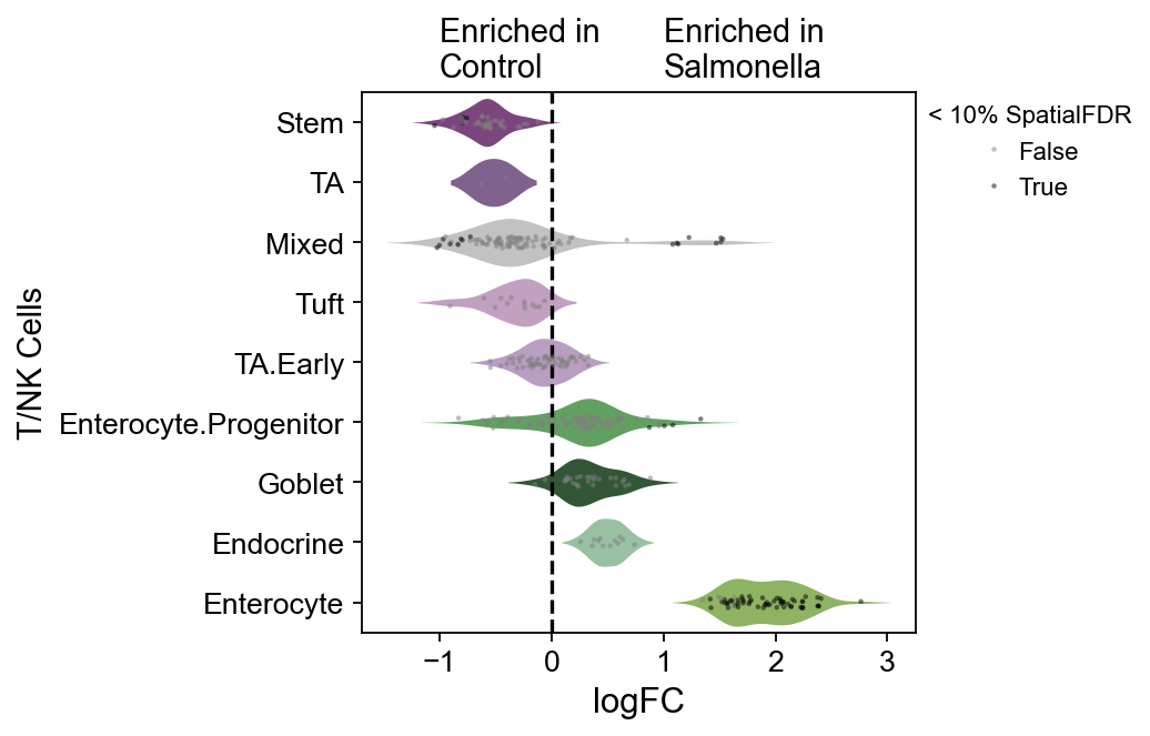
Text(1, -0.75, 'Enriched in\nSalmonella')
总结#
在本教程中,我们学习了如何在OmicVerse中进行全面的单细胞差异表达分析。
dct_obj_old=ov.single.DCT( adata, condition='condition', ctrl_group='Control', test_group='Salmonella', cell_type_key='cell_label', method='milo', sample_key='batch', use_rep='X_harmony')
✅ Differential cell type abundance analysis initialized
📊 DCT analysis using milo method
📊 Condition: condition, Control group: Control, Test group: Salmonella
computing neighbors
    finished: added to `.uns['neighbors']`
    `.obsp['distances']`, distances for each pair of neighbors
    `.obsp['connectivities']`, weighted adjacency matrix (0:00:07)
dct_obj_old.run()
✅ milo DCT analysis completed
# 高级用法:批量效应校正的DEG
adata_corrected = ov.pp.harmony(adata)
de_results_corrected = ov.single.DEG(adata_corrected, groupby='cell_type')
Text(1, -0.75, 'Enriched in\nSalmonella')