
Preprocessing the data of scRNA-seq with omicverse[CPU-GPU-mixed]#
The count table, a numeric matrix of genes × cells, is the basic input data structure in the analysis of single-cell RNA-sequencing data. A common preprocessing step is to adjust the counts for variable sampling efficiency and to transform them so that the variance is similar across the dynamic range.
Suitable methods to preprocess the scRNA-seq is important. Here, we introduce some preprocessing step to help researchers can perform downstream analysis easyier.
User can compare our tutorial with scanpy’tutorial to learn how to use omicverse well
Colab 可重现性:https://colab.research.google.com/drive/1DXLSls_ppgJmAaZTUvqazNC_E7EDCxUe?usp=sharing
import scanpy as sc
import omicverse as ov
ov.plot_set(font_path='Arial')

# Enable auto-reload for development
%load_ext autoreload
%autoreload 2
🔬 Starting plot initialization...
Using already downloaded Arial font from: /tmp/omicverse_arial.ttf
Registered as: Arial
🧬 Detecting GPU devices…
✅ NVIDIA CUDA GPUs detected: 1
• [CUDA 0] NVIDIA H100 80GB HBM3
      Memory: 79.1 GB | Compute: 9.0

   ____            _     _    __
  / __ \____ ___  (_)___| |  / /__  _____________
 / / / / __ `__ \/ / ___/ | / / _ \/ ___/ ___/ _ \
/ /_/ / / / / / / / /__ | |/ /  __/ /  (__  )  __/
\____/_/ /_/ /_/_/\___/ |___/\___/_/  /____/\___/

🔖 Version: 2.1.2rc1   📚 Tutorials: https://omicverse.readthedocs.io/
✅ plot_set complete.
备注
“When OmicVerse is upgraded to version > 1.7.0, it supports CPU–GPU mixed acceleration without requiring rapids_singlecell as a dependency—enjoy faster single-cell analysis!”
ov.settings.cpu_gpu_mixed_init()
CPU-GPU mixed mode activated
Available GPU accelerators: CUDA
用 omicverse 自带的 PBMC 8k 数据集(ov.datasets.pbmc8k() 首次会自动下载,之后走缓存):
# Load PBMC 8k from omicverse's bundled datasets
adata = ov.datasets.pbmc8k()
adata.var_names_make_unique()
adata.obs_names_make_unique()
adata
🩸 Downloading PBMC 8k dataset
Using Stanford mirror for pbmc8k
⚠️ File ./data/pbmc8k.h5ad already exists
 Loading data from ./data/pbmc8k.h5ad
✅ Successfully loaded: 7750 cells × 20939 genes
AnnData object with n_obs × n_vars = 7750 × 20939
    obs: 'kit', 'tissue_ontology_term_id', 'tissue_type', 'assay_ontology_term_id', 'disease_ontology_term_id', 'cell_type_ontology_term_id', 'self_reported_ethnicity_ontology_term_id', 'development_stage_ontology_term_id', 'sex_ontology_term_id', 'donor_id', 'suspension_type', 'predicted_celltype', 'is_primary_data', 'cell_type', 'assay', 'disease', 'sex', 'tissue', 'self_reported_ethnicity', 'development_stage', 'observation_joinid'
    var: 'gene_name', 'feature_name', 'feature_reference', 'feature_biotype', 'feature_length', 'feature_type'
    obsm: 'UMAP', 'X_pca', 'X_umap'
Preprocessing#
Quantity control#
For single-cell data, we require quality control prior to analysis, including the removal of cells containing double cells, low-expressing cells, and low-expressing genes. In addition to this, we need to filter based on mitochondrial gene ratios, number of transcripts, number of genes expressed per cell, cellular Complexity, etc. For a detailed description of the different QCs please see the document: https://hbctraining.github.io/scRNA-seq/lessons/04_SC_quality_control.html
注意
if the version of omicverse larger than 1.6.4, the doublets_method can be set between scrublet and sccomposite.
COMPOSITE (COMpound POiSson multIplet deTEction model) is a computational tool for multiplet detection in both single-cell single-omics and multiomics settings. It has been implemented as an automated pipeline and is available as both a cloud-based application with a user-friendly interface and a Python package.
Hu, H., Wang, X., Feng, S. et al. A unified model-based framework for doublet or multiplet detection in single-cell multiomics data. Nat Commun 15, 5562 (2024). https://doi.org/10.1038/s41467-024-49448-x
%%time
adata=ov.pp.qc(
    adata,
    tresh={'mito_perc': 0.2, 'nUMIs': 500, 'detected_genes': 250},
    doublets_method='scrublet',
    batch_key=None,
    filter_doublets=True,
)
adata
⚙️ Using CPU/GPU mixed mode for QC...
NVIDIA CUDA GPUs detected:
📊 [CUDA 0] NVIDIA H100 80GB HBM3
    ------------------------------ 1109/81559 MiB (1.4%)

🔍 Quality Control Analysis (CPU-GPU Mixed):
   Dataset shape: 7,750 cells × 20,939 genes
   QC mode: seurat
   Doublet detection: scrublet
   Auto-detected mitochondrial prefix: 'MT-'
   Mitochondrial genes: MT-

📊 Step 1: Calculating QC Metrics

   ✓ Gene Family Detection:
   ┌──────────────────────────────┬────────────────────┬────────────────────┐
   │ Gene Family                  │ Genes Found        │ Detection Method   │
   ├──────────────────────────────┼────────────────────┼────────────────────┤
   │ Mitochondrial                │ 13                 │ Auto (MT-)         │
   ├──────────────────────────────┼────────────────────┼────────────────────┤
   │ Ribosomal                    │ 99                 │ Auto (RPS/RPL)     │
   ├──────────────────────────────┼────────────────────┼────────────────────┤
   │ Hemoglobin                   │ 7                  │ Auto (regex)       │
   └──────────────────────────────┴────────────────────┴────────────────────┘

   ✓ QC Metrics Summary:
   ┌─────────────────────────┬────────────────────┬─────────────────────────┐
   │ Metric                  │ Mean               │ Range (Min - Max)       │
   ├─────────────────────────┼────────────────────┼─────────────────────────┤
   │ nUMIs                   │ 5454               │ 497 - 34434             │
   ├─────────────────────────┼────────────────────┼─────────────────────────┤
   │ Detected Genes          │ 2071               │ 35 - 6427               │
   ├─────────────────────────┼────────────────────┼─────────────────────────┤
   │ Mitochondrial %         │ 2.9%               │ 0.0% - 97.2%            │
   ├─────────────────────────┼────────────────────┼─────────────────────────┤
   │ Ribosomal %             │ 20.4%              │ 0.1% - 52.8%            │
   ├─────────────────────────┼────────────────────┼─────────────────────────┤
   │ Hemoglobin %            │ 0.0%               │ 0.0% - 0.3%             │
   └─────────────────────────┴────────────────────┴─────────────────────────┘

🔧 Step 2: Quality Filtering (SEURAT)
   Thresholds: mito≤0.2, nUMIs≥500, genes≥250
   📊 Seurat Filter Results:
     • nUMIs filter (≥500): 5 cells failed (0.1%)
     • Genes filter (≥250): 16 cells failed (0.2%)
     • Mitochondrial filter (≤0.2): 40 cells failed (0.5%)
   ✓ Combined QC filters: 7,698 cells kept (99.3%)

🎯 Step 3: Final Filtering
   Parameters: min_genes=200, min_cells=3
   Ratios: max_genes_ratio=1, max_cells_ratio=1
✓ Final filtering: 0 cells, 10 genes removed

🔍 Step 4: Doublet Detection
   ⚠️  Note: 'scrublet' detection is legacy and may not work optimally
   💡 Consider using 'doublets_method=scdblfinder' (default) for better results
   🔍 Running scrublet doublet detection...

🔍 Running Scrublet Doublet Detection:
   Mode: cpu-gpu-mixed
   Computing doublet prediction using Scrublet algorithm
   🔍 Filtering genes and cells...
🔍 Filtering genes...
   Parameters: min_cells≥3
✓ Filtered: 0 genes removed
🔍 Filtering cells...
   Parameters: min_genes≥3
✓ Filtered: 0 cells removed
   🔍 Normalizing data and selecting highly variable genes...

🔍 Count Normalization:
   Target sum: median
   Exclude highly expressed: False

✅ Count Normalization Completed Successfully!
   ✓ Processed: 7,698 cells × 20,929 genes
   ✓ Runtime: 0.06s
🔍 Highly Variable Genes Selection:
   Method: seurat
✅ HVG Selection Completed Successfully!
   ✓ Selected: 1,837 highly variable genes out of 20,929 total (8.8%)
   ✓ Results added to AnnData object:
     • 'highly_variable': Boolean vector (adata.var)
     • 'means': Float vector (adata.var)
     • 'dispersions': Float vector (adata.var)
     • 'dispersions_norm': Float vector (adata.var)
   🔍 Simulating synthetic doublets...
🔍 Normalizing observed and simulated data...

🔍 Count Normalization:
   Target sum: 1000000.0
   Exclude highly expressed: False

✅ Count Normalization Completed Successfully!
   ✓ Processed: 7,698 cells × 1,837 genes
   ✓ Runtime: 0.00s

🔍 Count Normalization:
   Target sum: 1000000.0
   Exclude highly expressed: False

✅ Count Normalization Completed Successfully!
   ✓ Processed: 15,396 cells × 1,837 genes
   ✓ Runtime: 0.05s
🔍 Embedding transcriptomes using PCA...

Using CUDA device: NVIDIA H100 80GB HBM3
✅ Using built-in torch_pca for GPU-accelerated PCA
   🚀 Using torch_pca PCA for CUDA GPU acceleration in scrublet
   🚀 torch_pca PCA backend: CUDA GPU acceleration (scrublet, supports sparse)
   📊 Scrublet PCA input data type - X_obs: ndarray, shape: (7698, 1837), dtype: float64
   📊 Scrublet PCA input data type - X_sim: ndarray, shape: (15396, 1837), dtype: float64
🔍 Calculating doublet scores...
🔍 Calling doublets with threshold detection...
   📊 Automatic threshold: 0.438
   📈 Detected doublet rate: 0.3%
   🔍 Detectable doublet fraction: 36.0%
   📊 Overall doublet rate comparison:
     • Expected: 5.0%
     • Estimated: 0.8%

✅ Scrublet Analysis Completed Successfully!
   ✓ Results added to AnnData object:
     • 'doublet_score': Doublet scores (adata.obs)
     • 'predicted_doublet': Boolean predictions (adata.obs)
     • 'scrublet': Parameters and metadata (adata.uns)
   ✓ Scrublet completed: 21 doublets removed (0.3%)
╭─ SUMMARY: qc ──────────────────────────────────────────────────────╮
│  Duration: 5.0037s                                                 │
│  Shape:    7,750 x 20,939 (Unchanged)                              │
│                                                                    │
│  CHANGES DETECTED                                                  │
│  ────────────────                                                  │
│  ● OBS    │ ✚ cell_complexity (float)                              │
│           │ ✚ detected_genes (int)                                 │
│           │ ✚ hb_perc (float)                                      │
│           │ ✚ mito_perc (float)                                    │
│           │ ✚ nUMIs (float)                                        │
│           │ ✚ passing_mt (bool)                                    │
│           │ ✚ passing_nUMIs (bool)                                 │
│           │ ✚ passing_ngenes (bool)                                │
│           │ ✚ passing_qc_step1 (bool)                              │
│           │ ✚ ribo_perc (float)                                    │
│                                                                    │
│  ● VAR    │ ✚ hb (bool)                                            │
│           │ ✚ mt (bool)                                            │
│           │ ✚ ribo (bool)                                          │
│                                                                    │
╰────────────────────────────────────────────────────────────────────╯
CPU times: user 5.22 s, sys: 2.69 s, total: 7.92 s
Wall time: 5.15 s
AnnData object with n_obs × n_vars = 7677 × 20929
    obs: 'kit', 'tissue_ontology_term_id', 'tissue_type', 'assay_ontology_term_id', 'disease_ontology_term_id', 'cell_type_ontology_term_id', 'self_reported_ethnicity_ontology_term_id', 'development_stage_ontology_term_id', 'sex_ontology_term_id', 'donor_id', 'suspension_type', 'predicted_celltype', 'is_primary_data', 'cell_type', 'assay', 'disease', 'sex', 'tissue', 'self_reported_ethnicity', 'development_stage', 'observation_joinid', 'nUMIs', 'mito_perc', 'ribo_perc', 'hb_perc', 'detected_genes', 'cell_complexity', 'passing_mt', 'passing_nUMIs', 'passing_ngenes', 'passing_qc_step1', 'doublet_score', 'predicted_doublet'
    var: 'gene_name', 'feature_name', 'feature_reference', 'feature_biotype', 'feature_length', 'feature_type', 'mt', 'ribo', 'hb'
    uns: 'scrublet', 'status', 'status_args', 'REFERENCE_MANU', '_ov_provenance'
    obsm: 'UMAP', 'X_pca', 'X_umap'
可选的双细胞后端 — py-DoubletFinder#
除了 scrublet 和 sccomposite,ov.pp.qc 现在支持 doublets_method='doubletfinder' —— 这是对经典 R 语言 DoubletFinder 算法(McGinnis 等, Cell Systems 2019)的纯 Python 重现:相同的 pANN 算法、在匹配的 PCA 输入下可与 R 结果做到浮点精度一致;同时借助 scipy.spatial.distance.cdist + np.argpartition top-k,pANN 核心计算比 R 更快。
pip install pydoubletfinder
使用方式只是切换一下 doublets_method 参数:
%%time
adata_df = ov.pp.qc(
    adata.copy(),
    tresh={'mito_perc': 0.2, 'nUMIs': 500, 'detected_genes': 250},
    doublets_method='doubletfinder',   # ← new backend (install: pip install pydoubletfinder)
    batch_key=None,
    filter_doublets=True,
)
print(adata_df)
print("doublet score column:", [c for c in adata_df.obs.columns if 'doublet' in c][:5])
可选的双细胞后端 — py-scDblFinder#
ov.pp.qc 还支持 doublets_method='scdblfinder' —— 这是对 R 语言 scDblFinder(Germain 等, F1000Research 2022)的纯 Python 重现。它用 xgboost 分类器在 kNN + cxds 特征上训练,和 scrublet(模拟邻居比例)、DoubletFinder(pANN)是互补的范式。
pip install pyscdblfinder
与 R 参考实现在 pbmc3k 上的分类一致率约为 96%;xgboost 跨语言打分无法做到 bit-for-bit 一致的原因见 pyscdblfinder README。
%%time
adata_scdbl = ov.pp.qc(
    adata.copy(),
    tresh={'mito_perc': 0.2, 'nUMIs': 500, 'detected_genes': 250},
    doublets_method='scdblfinder',   # ← new backend (install: pip install pyscdblfinder)
    batch_key=None,
    filter_doublets=True,
)
print(adata_scdbl)
print("score column:", [c for c in adata_scdbl.obs.columns if 'doublet' in c.lower() or 'scdbl' in c.lower()][:5])
High variable Gene Detection#
Here we try to use Pearson’s method to calculate highly variable genes. This is the method that is proposed to be superior to ordinary normalisation. See Article in Nature Method for details.
normalize|HVGs:We use | to control the preprocessing step, | before for the normalisation step, either shiftlog or pearson, and | after for the highly variable gene calculation step, either pearson or seurat. Our default is shiftlog|pearson.
if you use
mode=shiftlog|pearsonyou need to settarget_sum=50*1e4, more people like to setarget_sum=1e4, we test the result think 50*1e4 will be betterif you use
mode=pearson|pearson, you don’t need to settarget_sum
注意
if the version of omicverse lower than 1.4.13, the mode can only be set between scanpy and pearson.
%%time
adata=ov.pp.preprocess(
    adata,mode='shiftlog|pearson',n_HVGs=2000,
    target_sum=50*1e4,identify_robust=True,
)
adata
🔍 [2026-04-20 17:33:04] Running preprocessing in 'cpu-gpu-mixed' mode...
Begin robust gene identification
    After filtration, 20929/20929 genes are kept.
    Among 20929 genes, 20050 genes are robust.
✅ Robust gene identification completed successfully.
Begin size normalization: shiftlog and HVGs selection pearson
🔍 Count Normalization:
   Target sum: 500000.0
   Exclude highly expressed: True
   Max fraction threshold: 0.2
⚠️ Excluding 1 highly-expressed genes from normalization computation
   Excluded genes: ['IGLV3-21']

✅ Count Normalization Completed Successfully!
   ✓ Processed: 7,677 cells × 20,050 genes
   ✓ Runtime: 0.59s
🔍 Highly Variable Genes Selection (Experimental):
   Method: pearson_residuals
   Target genes: 2,000
   Theta (overdispersion): 100
✅ Experimental HVG Selection Completed Successfully!
   ✓ Selected: 2,000 highly variable genes out of 20,050 total (10.0%)
   ✓ Results added to AnnData object:
     • 'highly_variable': Boolean vector (adata.var)
     • 'highly_variable_rank': Float vector (adata.var)
     • 'highly_variable_nbatches': Int vector (adata.var)
     • 'highly_variable_intersection': Boolean vector (adata.var)
     • 'means': Float vector (adata.var)
     • 'variances': Float vector (adata.var)
     • 'residual_variances': Float vector (adata.var)
    Time to analyze data in cpu: 1.87 seconds.
✅ Preprocessing completed successfully.
    Added:
        'highly_variable_features', boolean vector (adata.var)
        'means', float vector (adata.var)
        'variances', float vector (adata.var)
        'residual_variances', float vector (adata.var)
        'counts', raw counts layer (adata.layers)
    End of size normalization: shiftlog and HVGs selection pearson

╭─ SUMMARY: preprocess ──────────────────────────────────────────────╮
│  Duration: 2.3753s                                                 │
│  Shape:    7,677 x 20,929 -> 7,677 x 20,050                        │
│                                                                    │
│  CHANGES DETECTED                                                  │
│  ────────────────                                                  │
│  ● VAR    │ ✚ highly_variable (bool)                               │
│           │ ✚ highly_variable_features (bool)                      │
│           │ ✚ highly_variable_rank (float)                         │
│           │ ✚ means (float)                                        │
│           │ ✚ n_cells (int)                                        │
│           │ ✚ percent_cells (float)                                │
│           │ ✚ residual_variances (float)                           │
│           │ ✚ robust (bool)                                        │
│           │ ✚ variances (float)                                    │
│                                                                    │
│  ● UNS    │ ✚ history_log                                          │
│           │ ✚ hvg                                                  │
│           │ ✚ log1p                                                │
│                                                                    │
│  ● LAYERS │ ✚ counts (sparse matrix, 7677x20050)                   │
│                                                                    │
╰────────────────────────────────────────────────────────────────────╯
CPU times: user 2.81 s, sys: 1.3 s, total: 4.12 s
Wall time: 2.38 s
AnnData object with n_obs × n_vars = 7677 × 20050
    obs: 'kit', 'tissue_ontology_term_id', 'tissue_type', 'assay_ontology_term_id', 'disease_ontology_term_id', 'cell_type_ontology_term_id', 'self_reported_ethnicity_ontology_term_id', 'development_stage_ontology_term_id', 'sex_ontology_term_id', 'donor_id', 'suspension_type', 'predicted_celltype', 'is_primary_data', 'cell_type', 'assay', 'disease', 'sex', 'tissue', 'self_reported_ethnicity', 'development_stage', 'observation_joinid', 'nUMIs', 'mito_perc', 'ribo_perc', 'hb_perc', 'detected_genes', 'cell_complexity', 'passing_mt', 'passing_nUMIs', 'passing_ngenes', 'passing_qc_step1', 'doublet_score', 'predicted_doublet'
    var: 'gene_name', 'feature_name', 'feature_reference', 'feature_biotype', 'feature_length', 'feature_type', 'mt', 'ribo', 'hb', 'n_cells', 'percent_cells', 'robust', 'highly_variable_features', 'means', 'variances', 'residual_variances', 'highly_variable_rank', 'highly_variable'
    uns: 'scrublet', 'status', 'status_args', 'REFERENCE_MANU', '_ov_provenance', 'history_log', 'log1p', 'hvg'
    obsm: 'UMAP', 'X_pca', 'X_umap'
    layers: 'counts'
You can use recover_counts to recover the raw counts after normalize and log1p
adata[:,'CD3D'].to_df().T
      TGAGCCGTCGATAGAA-1_10X_5-rep1  TACACGACAGGACGTA-1_10X_5-rep1  \
gene
CD3D                            0.0                            0.0

      GAAGCAGCAGCTGTGC-1_10X_5-rep1  CTCACACAGAGCCCAA-1_10X_5-rep1  \
gene
CD3D                            0.0                       6.131753

      CTCGTCAGTGATAAAC-1_10X_5-rep1  TGTATTCTCAGCGATT-1_10X_5-rep1  \
gene
CD3D                            0.0                       5.498595

      GTTACAGCAGCTCGAC-1_10X_5-rep1  GTTAAGCGTCTGGAGA-1_10X_5-rep1  \
gene
CD3D                            0.0                            0.0

      TTGGCAAAGCCGTCGT-1_10X_5-rep1  CCTTCCCGTCTAGTGT-1_10X_5-rep1  ...  \
gene                                                                ...
CD3D                            0.0                            0.0  ...

      CACCTTGAGTTACCCA-1_10X_5-rep1  GCTCCTAAGTACTTGC-1_10X_5-rep1  \
gene
CD3D                       5.766456                            0.0

      CTGCGGATCTGGAGCC-1_10X_5-rep1  ATAGACCGTCAGTGGA-1_10X_5-rep1  \
gene
CD3D                            0.0                            0.0

      ACATCAGGTATTACCG-1_10X_5-rep1  TTAACTCGTTACGACT-1_10X_5-rep1  \
gene
CD3D                            0.0                            0.0

      TCGCGAGCATGGGACA-1_10X_5-rep1  GCGAGAAGTATTACCG-1_10X_5-rep1  \
gene
CD3D                            0.0                            0.0

      CACCACTTCTTCGAGA-1_10X_5-rep1  AGGGATGTCCAGATCA-1_10X_5-rep1
gene
CD3D                            0.0                            0.0

[1 rows x 7677 columns]
adata[:,'CD3D'].to_df(layer='counts').T
      TGAGCCGTCGATAGAA-1_10X_5-rep1  TACACGACAGGACGTA-1_10X_5-rep1  \
gene
CD3D                            0.0                            0.0

      GAAGCAGCAGCTGTGC-1_10X_5-rep1  CTCACACAGAGCCCAA-1_10X_5-rep1  \
gene
CD3D                            0.0                            4.0

      CTCGTCAGTGATAAAC-1_10X_5-rep1  TGTATTCTCAGCGATT-1_10X_5-rep1  \
gene
CD3D                            0.0                            3.0

      GTTACAGCAGCTCGAC-1_10X_5-rep1  GTTAAGCGTCTGGAGA-1_10X_5-rep1  \
gene
CD3D                            0.0                            0.0

      TTGGCAAAGCCGTCGT-1_10X_5-rep1  CCTTCCCGTCTAGTGT-1_10X_5-rep1  ...  \
gene                                                                ...
CD3D                            0.0                            0.0  ...

      CACCTTGAGTTACCCA-1_10X_5-rep1  GCTCCTAAGTACTTGC-1_10X_5-rep1  \
gene
CD3D                            3.0                            0.0

      CTGCGGATCTGGAGCC-1_10X_5-rep1  ATAGACCGTCAGTGGA-1_10X_5-rep1  \
gene
CD3D                            0.0                            0.0

      ACATCAGGTATTACCG-1_10X_5-rep1  TTAACTCGTTACGACT-1_10X_5-rep1  \
gene
CD3D                            0.0                            0.0

      TCGCGAGCATGGGACA-1_10X_5-rep1  GCGAGAAGTATTACCG-1_10X_5-rep1  \
gene
CD3D                            0.0                            0.0

      CACCACTTCTTCGAGA-1_10X_5-rep1  AGGGATGTCCAGATCA-1_10X_5-rep1
gene
CD3D                            0.0                            0.0

[1 rows x 7677 columns]
X_counts_recovered, size_factors_sub=ov.pp.recover_counts(adata.X, 50*1e4, 50*1e5, log_base=None,
                                                          chunk_size=10000)
adata.layers['recover_counts']=X_counts_recovered
adata[:,'CD3D'].to_df(layer='recover_counts').T
      TGAGCCGTCGATAGAA-1_10X_5-rep1  TACACGACAGGACGTA-1_10X_5-rep1  \
gene
CD3D                              0                              0

      GAAGCAGCAGCTGTGC-1_10X_5-rep1  CTCACACAGAGCCCAA-1_10X_5-rep1  \
gene
CD3D                              0                              3

      CTCGTCAGTGATAAAC-1_10X_5-rep1  TGTATTCTCAGCGATT-1_10X_5-rep1  \
gene
CD3D                              0                              2

      GTTACAGCAGCTCGAC-1_10X_5-rep1  GTTAAGCGTCTGGAGA-1_10X_5-rep1  \
gene
CD3D                              0                              0

      TTGGCAAAGCCGTCGT-1_10X_5-rep1  CCTTCCCGTCTAGTGT-1_10X_5-rep1  ...  \
gene                                                                ...
CD3D                              0                              0  ...

      CACCTTGAGTTACCCA-1_10X_5-rep1  GCTCCTAAGTACTTGC-1_10X_5-rep1  \
gene
CD3D                              3                              0

      CTGCGGATCTGGAGCC-1_10X_5-rep1  ATAGACCGTCAGTGGA-1_10X_5-rep1  \
gene
CD3D                              0                              0

      ACATCAGGTATTACCG-1_10X_5-rep1  TTAACTCGTTACGACT-1_10X_5-rep1  \
gene
CD3D                              0                              0

      TCGCGAGCATGGGACA-1_10X_5-rep1  GCGAGAAGTATTACCG-1_10X_5-rep1  \
gene
CD3D                              0                              0

      CACCACTTCTTCGAGA-1_10X_5-rep1  AGGGATGTCCAGATCA-1_10X_5-rep1
gene
CD3D                              0                              0

[1 rows x 7677 columns]
Set the .raw attribute of the AnnData object to the normalized and logarithmized raw gene expression for later use in differential testing and visualizations of gene expression. This simply freezes the state of the AnnData object.
%%time
adata.raw = adata
adata = adata[:, adata.var.highly_variable_features]
adata
CPU times: user 36.6 ms, sys: 64.9 ms, total: 102 ms
Wall time: 102 ms
View of AnnData object with n_obs × n_vars = 7677 × 2000
    obs: 'kit', 'tissue_ontology_term_id', 'tissue_type', 'assay_ontology_term_id', 'disease_ontology_term_id', 'cell_type_ontology_term_id', 'self_reported_ethnicity_ontology_term_id', 'development_stage_ontology_term_id', 'sex_ontology_term_id', 'donor_id', 'suspension_type', 'predicted_celltype', 'is_primary_data', 'cell_type', 'assay', 'disease', 'sex', 'tissue', 'self_reported_ethnicity', 'development_stage', 'observation_joinid', 'nUMIs', 'mito_perc', 'ribo_perc', 'hb_perc', 'detected_genes', 'cell_complexity', 'passing_mt', 'passing_nUMIs', 'passing_ngenes', 'passing_qc_step1', 'doublet_score', 'predicted_doublet'
    var: 'gene_name', 'feature_name', 'feature_reference', 'feature_biotype', 'feature_length', 'feature_type', 'mt', 'ribo', 'hb', 'n_cells', 'percent_cells', 'robust', 'highly_variable_features', 'means', 'variances', 'residual_variances', 'highly_variable_rank', 'highly_variable'
    uns: 'scrublet', 'status', 'status_args', 'REFERENCE_MANU', '_ov_provenance', 'history_log', 'log1p', 'hvg'
    obsm: 'UMAP', 'X_pca', 'X_umap'
    layers: 'counts', 'recover_counts'
Principal component analysis#
In contrast to scanpy, we do not directly scale the variance of the original expression matrix, but store the results of the variance scaling in the layer, due to the fact that scale may cause changes in the data distribution, and we have not found scale to be meaningful in any scenario other than a principal component analysis
%%time
ov.pp.scale(adata)
adata
╭─ SUMMARY: scale ───────────────────────────────────────────────────╮
│  Duration: 0.7899s                                                 │
│  Shape:    7,677 x 2,000 (Unchanged)                               │
│                                                                    │
│  CHANGES DETECTED                                                  │
│  ────────────────                                                  │
│  ● LAYERS │ ✚ scaled (array, 7677x2000)                            │
│                                                                    │
╰────────────────────────────────────────────────────────────────────╯
CPU times: user 595 ms, sys: 260 ms, total: 854 ms
Wall time: 792 ms
AnnData object with n_obs × n_vars = 7677 × 2000
    obs: 'kit', 'tissue_ontology_term_id', 'tissue_type', 'assay_ontology_term_id', 'disease_ontology_term_id', 'cell_type_ontology_term_id', 'self_reported_ethnicity_ontology_term_id', 'development_stage_ontology_term_id', 'sex_ontology_term_id', 'donor_id', 'suspension_type', 'predicted_celltype', 'is_primary_data', 'cell_type', 'assay', 'disease', 'sex', 'tissue', 'self_reported_ethnicity', 'development_stage', 'observation_joinid', 'nUMIs', 'mito_perc', 'ribo_perc', 'hb_perc', 'detected_genes', 'cell_complexity', 'passing_mt', 'passing_nUMIs', 'passing_ngenes', 'passing_qc_step1', 'doublet_score', 'predicted_doublet'
    var: 'gene_name', 'feature_name', 'feature_reference', 'feature_biotype', 'feature_length', 'feature_type', 'mt', 'ribo', 'hb', 'n_cells', 'percent_cells', 'robust', 'highly_variable_features', 'means', 'variances', 'residual_variances', 'highly_variable_rank', 'highly_variable'
    uns: 'scrublet', 'status', 'status_args', 'REFERENCE_MANU', '_ov_provenance', 'history_log', 'log1p', 'hvg'
    obsm: 'UMAP', 'X_pca', 'X_umap'
    layers: 'counts', 'recover_counts', 'scaled'
If you want to perform pca in normlog layer, you can set layer=normlog, but we think scaled is necessary in PCA.
%%time
ov.pp.pca(adata,layer='scaled',n_pcs=50)
adata
🚀 Using GPU to calculate PCA...
NVIDIA CUDA GPUs detected:
📊 [CUDA 0] NVIDIA H100 80GB HBM3
    |----------------------------- 2889/81559 MiB (3.5%)
computing PCA🔍
    with n_comps=50
Using CUDA device: NVIDIA H100 80GB HBM3
✅ Using built-in torch_pca for GPU-accelerated PCA
   🚀 Using torch_pca PCA for CUDA GPU acceleration
   🚀 torch_pca PCA backend: CUDA GPU acceleration (supports sparse matrices)
   📊 PCA input data type: ArrayView, shape: (7677, 2000), dtype: float64
   🔧 solver_used_in_uns (planned): covariance_eigh
   🔧 PCA solver used: covariance_eigh
    finished✅ (0.35s)

╭─ SUMMARY: pca ─────────────────────────────────────────────────────╮
│  Duration: 0.3717s                                                 │
│  Shape:    7,677 x 2,000 (Unchanged)                               │
│                                                                    │
│  CHANGES DETECTED                                                  │
│  ────────────────                                                  │
│  ● UNS    │ ✚ pca                                                  │
│           │ └─ params: {'zero_center': True, 'use_highly_variable': Tr...│
│           │ ✚ scaled|original|cum_sum_eigenvalues                  │
│           │ ✚ scaled|original|pca_var_ratios                       │
│                                                                    │
│  ● OBSM   │ ✚ scaled|original|X_pca (array, 7677x50)               │
│                                                                    │
╰────────────────────────────────────────────────────────────────────╯
CPU times: user 196 ms, sys: 141 ms, total: 337 ms
Wall time: 373 ms
AnnData object with n_obs × n_vars = 7677 × 2000
    obs: 'kit', 'tissue_ontology_term_id', 'tissue_type', 'assay_ontology_term_id', 'disease_ontology_term_id', 'cell_type_ontology_term_id', 'self_reported_ethnicity_ontology_term_id', 'development_stage_ontology_term_id', 'sex_ontology_term_id', 'donor_id', 'suspension_type', 'predicted_celltype', 'is_primary_data', 'cell_type', 'assay', 'disease', 'sex', 'tissue', 'self_reported_ethnicity', 'development_stage', 'observation_joinid', 'nUMIs', 'mito_perc', 'ribo_perc', 'hb_perc', 'detected_genes', 'cell_complexity', 'passing_mt', 'passing_nUMIs', 'passing_ngenes', 'passing_qc_step1', 'doublet_score', 'predicted_doublet'
    var: 'gene_name', 'feature_name', 'feature_reference', 'feature_biotype', 'feature_length', 'feature_type', 'mt', 'ribo', 'hb', 'n_cells', 'percent_cells', 'robust', 'highly_variable_features', 'means', 'variances', 'residual_variances', 'highly_variable_rank', 'highly_variable'
    uns: 'scrublet', 'status', 'status_args', 'REFERENCE_MANU', '_ov_provenance', 'history_log', 'log1p', 'hvg', 'pca', 'scaled|original|pca_var_ratios', 'scaled|original|cum_sum_eigenvalues'
    obsm: 'UMAP', 'X_pca', 'X_umap', 'scaled|original|X_pca'
    varm: 'PCs', 'scaled|original|pca_loadings'
    layers: 'counts', 'recover_counts', 'scaled'
adata.obsm['X_pca']=adata.obsm['scaled|original|X_pca']
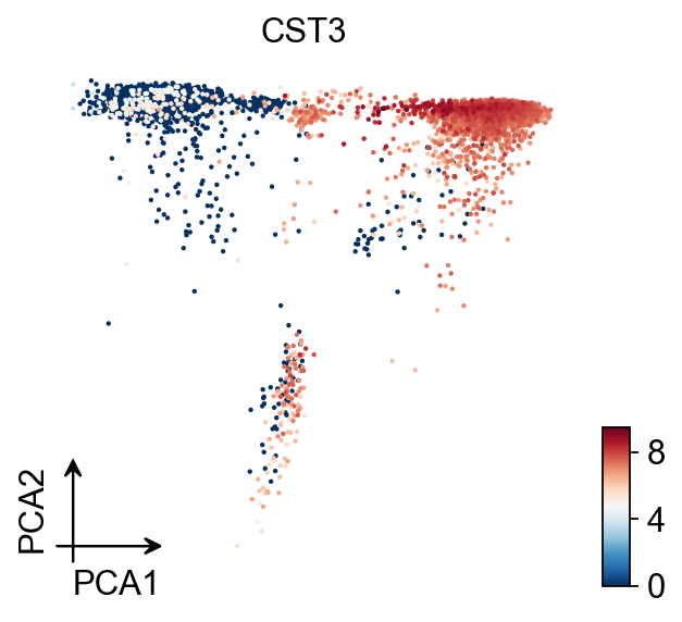
ov.pl.pca(adata,color='CST3')
X_pca converted to PCA to visualize and saved to adata.obsm['PCA']
if you want to use X_pca, please set convert=False
Embedding the neighborhood graph#
We suggest embedding the graph in two dimensions using UMAP (McInnes et al., 2018), see below. It is potentially more faithful to the global connectivity of the manifold than tSNE, i.e., it better preserves trajectories. In some ocassions, you might still observe disconnected clusters and similar connectivity violations. They can usually be remedied by running:
%%time
ov.pp.neighbors(adata, n_neighbors=15, n_pcs=50,
               use_rep='scaled|original|X_pca')
🚀 Using torch CPU/GPU mixed mode to calculate neighbors...
NVIDIA CUDA GPUs detected:
📊 [CUDA 0] NVIDIA H100 80GB HBM3
    |----------------------------- 2891/81559 MiB (3.5%)
🚀 Mixed mode default transformer: pyg

🔍 K-Nearest Neighbors Graph Construction:
   Mode: cpu-gpu-mixed
   Neighbors: 15
   Method: torch
   Metric: euclidean
   Transformer: pyg
   Representation: scaled|original|X_pca
   PCs used: 50
   🔍 Computing neighbor distances...
   💡 Using PyTorch Geometric KNN on cuda
   🔍 Computing connectivity matrix...
   💡 Using GPU-optimized connectivity computation
Using device: cuda
   ✓ Graph is fully connected

✅ KNN Graph Construction Completed Successfully!
   ✓ Processed: 7,677 cells with 15 neighbors each
   ✓ Results added to AnnData object:
     • 'neighbors': Neighbors metadata (adata.uns)
     • 'distances': Distance matrix (adata.obsp)
     • 'connectivities': Connectivity matrix (adata.obsp)

╭─ SUMMARY: neighbors ───────────────────────────────────────────────╮
│  Duration: 6.41s                                                   │
│  Shape:    7,677 x 2,000 (Unchanged)                               │
│                                                                    │
│  CHANGES DETECTED                                                  │
│  ────────────────                                                  │
│  ● UNS    │ ✚ neighbors                                            │
│           │ └─ params: {'n_neighbors': 15, 'method': 'torch', 'random_...│
│                                                                    │
│  ● OBSP   │ ✚ connectivities (sparse matrix, 7677x7677)            │
│           │ ✚ distances (sparse matrix, 7677x7677)                 │
│                                                                    │
╰────────────────────────────────────────────────────────────────────╯
CPU times: user 6.64 s, sys: 244 ms, total: 6.88 s
Wall time: 6.41 s
UMAP#
You also can use umap to visualize the neighborhood graph
%%time
ov.pp.umap(adata)
🔍 [2026-04-20 17:33:26] Running UMAP in 'cpu-gpu-mixed' mode...
🚀 Using torch GPU to calculate UMAP...
NVIDIA CUDA GPUs detected:
📊 [CUDA 0] NVIDIA H100 80GB HBM3
    |----------------------------- 2899/81559 MiB (3.6%)

🔍 UMAP Dimensionality Reduction:
   Mode: cpu-gpu-mixed
   Method: pumap
   Components: 2
   Min distance: 0.5
{'n_neighbors': 15, 'method': 'torch', 'random_state': 0, 'metric': 'euclidean', 'use_rep': 'scaled|original|X_pca', 'n_pcs': 50}
   ⚠️ Connectivities matrix was not computed with UMAP method
   🔍 Computing UMAP parameters...
   🔍 Computing UMAP embedding (Parametric PyTorch method)...
   Using device: cuda
   Dataset: 7677 samples × 50 features
   Batch size: 16384
   Learning rate: 0.001
   Total graph passes: 500 (split into 4 training epochs)
   Training parametric UMAP model...
============================================================
🚀 Parametric UMAP Training
============================================================
📊 Device: cuda
📈 Data shape: torch.Size([7677, 50])
🔗 Building UMAP graph...
♻️  Reusing cached GPU fuzzy graph (171174 edges)
🔢 Edge-SGD plan: 500 graph passes -> 4 training epochs x 340 batches of 16384
🏋️  Starting Training...
────────────────────────────────────────────────────────────
✓ New best loss: 0.2081
✓ New best loss: 0.1861
✓ New best loss: 0.1839
✓ New best loss: 0.1833

────────────────────────────────────────────────────────────
✅ Training Completed!
📉 Final best loss: 0.1833
============================================================

   💡 Using Parametric UMAP (PyTorch) on cuda

✅ UMAP Dimensionality Reduction Completed Successfully!
   ✓ Embedding shape: 7,677 cells × 2 dimensions
   ✓ Results added to AnnData object:
     • 'X_umap': UMAP coordinates (adata.obsm)
     • 'umap': UMAP parameters (adata.uns)
✅ UMAP completed successfully.

╭─ SUMMARY: umap ────────────────────────────────────────────────────╮
│  Duration: 6.2254s                                                 │
│  Shape:    7,677 x 2,000 (Unchanged)                               │
│                                                                    │
│  CHANGES DETECTED                                                  │
│  ────────────────                                                  │
│  ● UNS    │ ✚ umap                                                 │
│           │ └─ params: {'a': np.float64(0.5830300203414425), 'b': np.f...│
│                                                                    │
╰────────────────────────────────────────────────────────────────────╯
CPU times: user 6.1 s, sys: 2.02 s, total: 8.13 s
Wall time: 6.23 s
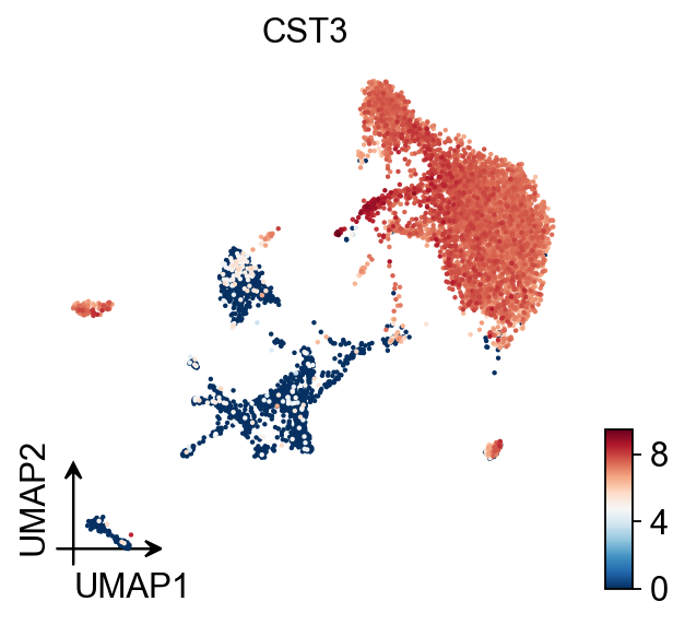
ov.pl.umap(adata,color='CST3')
X_umap converted to UMAP to visualize and saved to adata.obsm['UMAP']
if you want to use X_umap, please set convert=False
MDE#
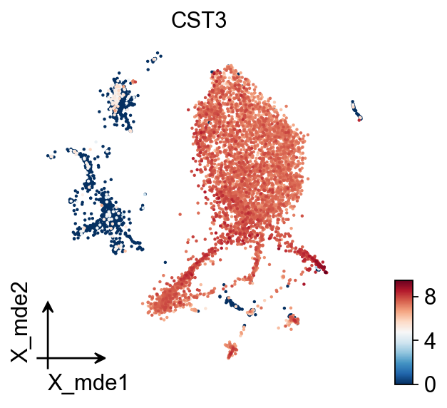
To visualize the PCA’s embeddings, we use the pymde package wrapper in omicverse. This is an alternative to UMAP that is GPU-accelerated.
ov.pp.mde(adata,embedding_dim=2,n_neighbors=15, basis='X_mde',
          n_pcs=50, use_rep='scaled|original|X_pca',)
🔍 MDE Dimensionality Reduction:
   Mode: cpu-gpu-mixed
   Embedding dimensions: 2
   Neighbors: 15
   Repulsive fraction: 0.7
   Using representation: scaled|original|X_pca
   Principal components: 50

Using CUDA device: NVIDIA H100 80GB HBM3
✅ Using built-in torch_pca for GPU-accelerated PCA
   🔍 Computing k-nearest neighbors graph...
🔍 Creating MDE embedding...
🔍 Optimizing embedding...
✅ MDE Dimensionality Reduction Completed Successfully!
   ✓ Embedding shape: 7,677 cells × 2 dimensions
   ✓ Runtime: 3.60s
   ✓ Results added to AnnData object:
     • 'X_mde': MDE coordinates (adata.obsm)
     • 'neighbors': Neighbors metadata (adata.uns)
     • 'distances': Distance matrix (adata.obsp)
     • 'connectivities': Connectivity matrix (adata.obsp)
ov.pl.embedding(adata,
                basis='X_mde',
                color='CST3',
                frameon='small')
TSNE#
%%time
ov.pp.tsne(adata,use_rep='scaled|original|X_pca')
⚙️ Using torch CPU/GPU mixed mode to calculate t-SNE...
NVIDIA CUDA GPUs detected:
📊 [CUDA 0] NVIDIA H100 80GB HBM3
    ------------------------------ 2327/81559 MiB (2.9%)

🔍 t-SNE Dimensionality Reduction:
   Mode: cpu-gpu-mixed
   Components: 2
   Perplexity: 30
   Learning rate: 1000
   🔍 Computing t-SNE with scikit-learn...
   💡 Using scikit-learn TSNE implementation
✅ t-SNE Dimensionality Reduction Completed Successfully!
   ✓ Embedding shape: 7,677 cells × 2 dimensions
   ✓ Results added to AnnData object:
     • 'X_tsne': t-SNE coordinates (adata.obsm)
     • 'tsne': t-SNE parameters (adata.uns)

╭─ SUMMARY: tsne ────────────────────────────────────────────────────╮
│  Duration: 53.4393s                                                │
│  Shape:    7,677 x 2,000 (Unchanged)                               │
│                                                                    │
│  CHANGES DETECTED                                                  │
│  ────────────────                                                  │
│  ● UNS    │ ✚ tsne                                                 │
│           │ └─ params: {'perplexity': 30, 'early_exaggeration': 12, 'l...│
│                                                                    │
│  ● OBSM   │ ✚ X_tsne (array, 7677x2)                               │
│                                                                    │
╰────────────────────────────────────────────────────────────────────╯
CPU times: user 11min 8s, sys: 2.51 s, total: 11min 11s
Wall time: 53.4 s
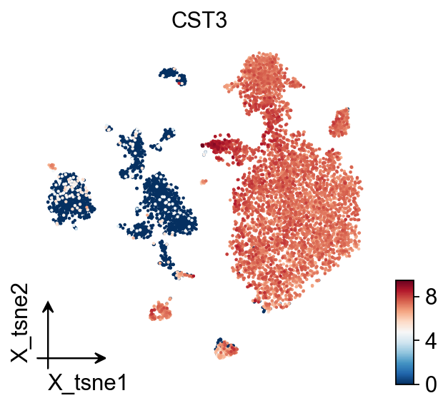
ov.pl.embedding(
    adata,
    basis='X_tsne',
    color='CST3',
    frameon='small'
)
SUDE#
SUDE, a scalable manifold learning method that uses uniform landmark sampling and constrained embedding to preserve both global structure and cluster separability, outperforming t-SNE, UMAP, and related methods across synthetic, real-world, and biomedical datasets.
Cite: Peng, D., Gui, Z., Wei, W. et al. Sampling-enabled scalable manifold learning unveils the discriminative cluster structure of high-dimensional data. Nat Mach Intell (2025). https://doi.org/10.1038/s42256-025-01112-9
%%time
ov.pp.sude(adata,use_rep='scaled|original|X_pca')
ov.pl.embedding(adata,
                basis='X_sude',
                color='CST3',
                frameon='small')
Score cell cyle#
In OmicVerse, we store both G1M/S and G2M genes into the function (both human and mouse), so you can run cell cycle analysis without having to manually enter cycle genes!
adata_raw=adata.raw.to_adata()
ov.pp.score_genes_cell_cycle(adata_raw,species='human')
WARNING: genes are not in var_names and ignored: Index(['MLF1IP'], dtype='object')
WARNING: genes are not in var_names and ignored: Index(['FAM64A', 'HN1'], dtype='object')
╭─ SUMMARY: score_genes_cell_cycle ──────────────────────────────────╮
│  Duration: 0.518s                                                  │
│  Shape:    7,677 x 20,050 (Unchanged)                              │
│                                                                    │
│  CHANGES DETECTED                                                  │
│  ────────────────                                                  │
│  ● OBS    │ ✚ G2M_score (float)                                    │
│           │ ✚ S_score (float)                                      │
│           │ ✚ phase (str)                                          │
│                                                                    │
╰────────────────────────────────────────────────────────────────────╯
ov.pl.mde(adata_raw,color='phase')
X_mde converted to MDE to visualize and saved to adata.obsm['MDE']
if you want to use X_mde, please set convert=False
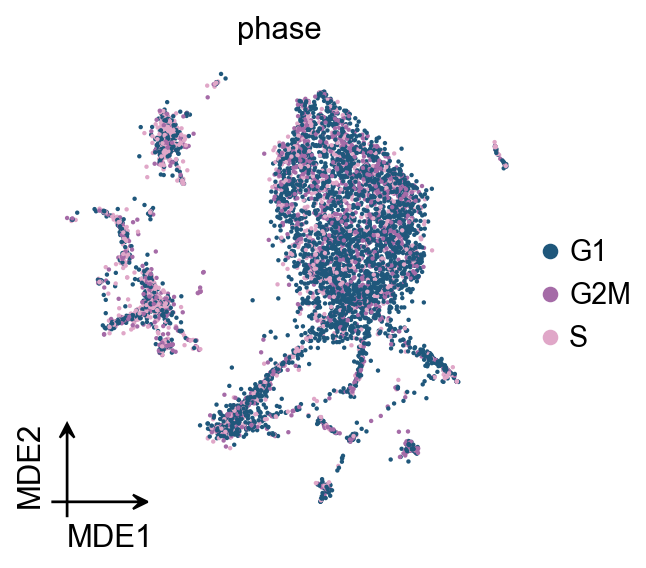
Clustering the neighborhood graph#
As with Seurat and many other frameworks, we recommend the Leiden graph-clustering method (community detection based on optimizing modularity) by Traag et al. (2018). 注意 that Leiden clustering directly clusters the neighborhood graph of cells, which we already computed in the previous section.
ov.pp.leiden(adata,resolution=1)
⚙️ Using torch CPU/GPU mixed mode to calculate Leiden...
NVIDIA CUDA GPUs detected:
📊 [CUDA 0] NVIDIA H100 80GB HBM3
    ------------------------------ 2327/81559 MiB (2.9%)
running Leiden clustering
finished (0.30s)
    found 20 clusters and added
    'leiden', the cluster labels (adata.obs, categorical)

╭─ SUMMARY: leiden ──────────────────────────────────────────────────╮
│  Duration: 0.3348s                                                 │
│  Shape:    7,677 x 2,000 (Unchanged)                               │
│                                                                    │
│  CHANGES DETECTED                                                  │
│  ────────────────                                                  │
│  ● OBS    │ ✚ leiden (category)                                    │
│                                                                    │
│  ● UNS    │ ✚ leiden                                               │
│           │ └─ params: {'resolution': 1, 'random_state': 0, 'n_iterati...│
│                                                                    │
╰────────────────────────────────────────────────────────────────────╯
自动选择 Leiden 分辨率#
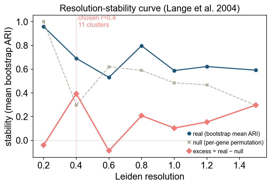
手动调 resolution 在探索阶段没问题,但要做可重现的 pipeline,用 ov.single.auto_resolution 自动选 —— 算法是 null-adjusted bootstrap-ARI stability(Lange, Roth, Braun & Buhmann, Neural Computation 2004):
对每个候选 resolution r:
在完整图上跑 Leiden → reference labels。
取
n_subsamples次随机 subsample,每次重跑 Leiden。对每次 bootstrap 算 ARI vs reference labels 在该 subsample 上的限制 →
stability_real(r)。对逐基因 permutation 后的 null 数据(彻底破坏所有细胞间相关性)跑同样的 PCA → kNN-graph → bootstrap pipeline →
stability_null(r)。选
argmax(stability_real - stability_null),约束n_clusters >= min_clusters。
null 校正是关键 —— 它把「小簇天然稳定」的 baseline 减掉,留下的才是真正反映生物学结构的稳定性。
# Suppress per-leiden SUMMARY boxes — only show the final scores table.
import io, contextlib
with contextlib.redirect_stdout(io.StringIO()):
    adata, best, scores = ov.single.auto_resolution(
        adata,
        resolutions=[0.2, 0.4, 0.6, 0.8, 1.0, 1.2, 1.5],
        n_subsamples=5,
        n_null_subsamples=3,
        random_state=0,
        key_added='leiden_auto',
    )
print(f'autoResolution chose r={best}')
scores
autoResolution chose r=0.4
            n_clusters  stability_real  stability_null  excess_stability  \
resolution
0.2                  8        0.959048        1.000000         -0.040952
0.4                 11        0.691287        0.297422          0.393865
0.6                 14        0.531035        0.619179         -0.088143
0.8                 15        0.796962        0.589003          0.207959
1.0                 20        0.588284        0.484690          0.103594
1.2                 22        0.622066        0.467593          0.154473
1.5                 25        0.591450        0.293998          0.297452

            std_real
resolution
0.2         0.013257
0.4         0.043664
0.6         0.022619
0.8         0.045211
1.0         0.039070
1.2         0.030341
1.5         0.019143
选择曲线把决策过程画出来:null(灰色)饱和到 1.0 的 r 段对应「一两个 trivial 大簇」,会被自动排除(excess 变负);null 塌掉之后 excess(红色)才有意义,excess 的峰值就是选中的 r。
ov.style()
ov.pl.auto_resolution_curve(adata)
🔬 Starting plot initialization...
🧬 Detecting GPU devices…
✅ NVIDIA CUDA GPUs detected: 1
    • [CUDA 0] NVIDIA H100 80GB HBM3
      Memory: 79.1 GB | Compute: 9.0
✅ plot_set complete.
<Axes: title={'center': 'Resolution-stability curve (Lange et al. 2004)'}, xlabel='Leiden resolution', ylabel='stability (mean bootstrap ARI)'>
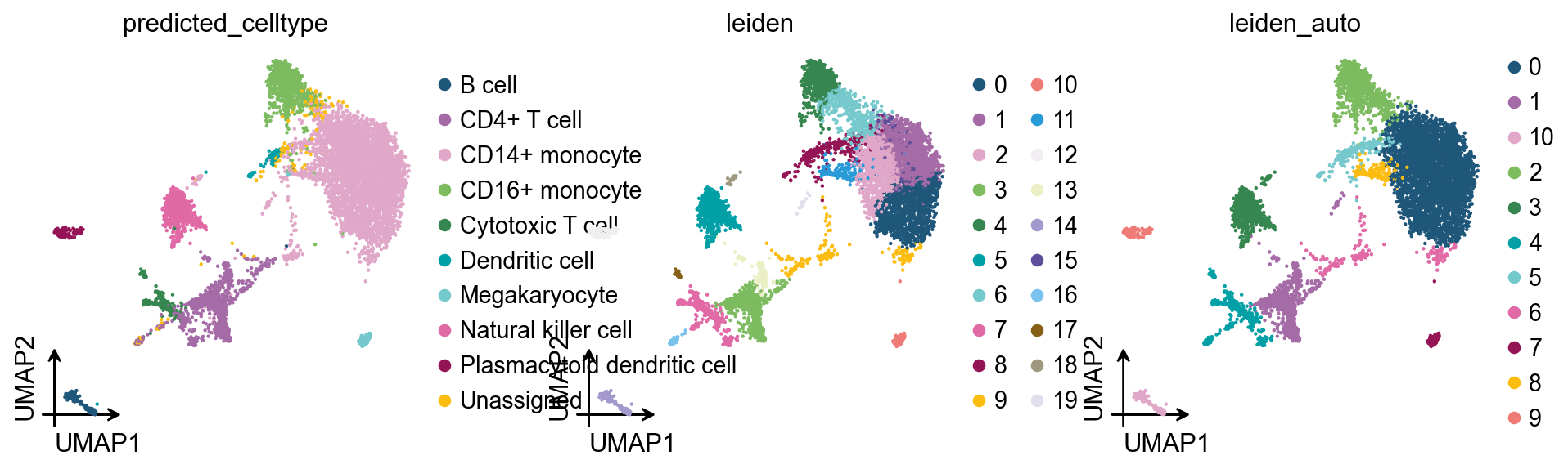
把自动选出的 cluster 投到 embedding 上,和数据集自带的 predicted_celltype 标注一起对比 —— 这正是 pbmc8k 适合做验证的原因:它带有 curated 好的 cell type 标注,可以直接打分。ARI/NMI 能量化 leiden_auto 和 predicted_celltype 的对齐程度。
ov.style()
from sklearn.metrics import adjusted_rand_score, normalized_mutual_info_score
ari = adjusted_rand_score(
    adata.obs['predicted_celltype'], adata.obs['leiden_auto'])
nmi = normalized_mutual_info_score(
    adata.obs['predicted_celltype'], adata.obs['leiden_auto'])
print(f'ARI(leiden_auto, predicted_celltype) = {ari:.3f}')
print(f'NMI(leiden_auto, predicted_celltype) = {nmi:.3f}')
ov.pl.umap(
    adata,
    color=['predicted_celltype', 'leiden', 'leiden_auto'],
    frameon='small',
    palette=ov.pl.sc_color,
    ncols=3,
)
🔬 Starting plot initialization...
🧬 Detecting GPU devices…
✅ NVIDIA CUDA GPUs detected: 1
    • [CUDA 0] NVIDIA H100 80GB HBM3
      Memory: 79.1 GB | Compute: 9.0
✅ plot_set complete.

ARI(leiden_auto, predicted_celltype) = 0.830
NMI(leiden_auto, predicted_celltype) = 0.807
X_umap converted to UMAP to visualize and saved to adata.obsm['UMAP']
if you want to use X_umap, please set convert=False
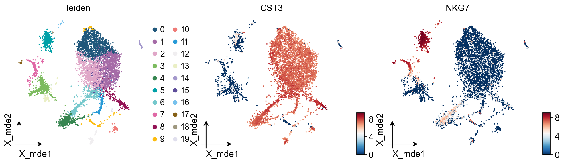
We redesigned the visualisation of embedding to distinguish it from scanpy’s embedding by adding the parameter fraemon='small', which causes the axes to be scaled with the colourbar
ov.pl.embedding(
    adata,
    basis='X_mde',
    color=['leiden', 'CST3', 'NKG7'],
    frameon='small',
    palette=ov.pl.sc_color
)
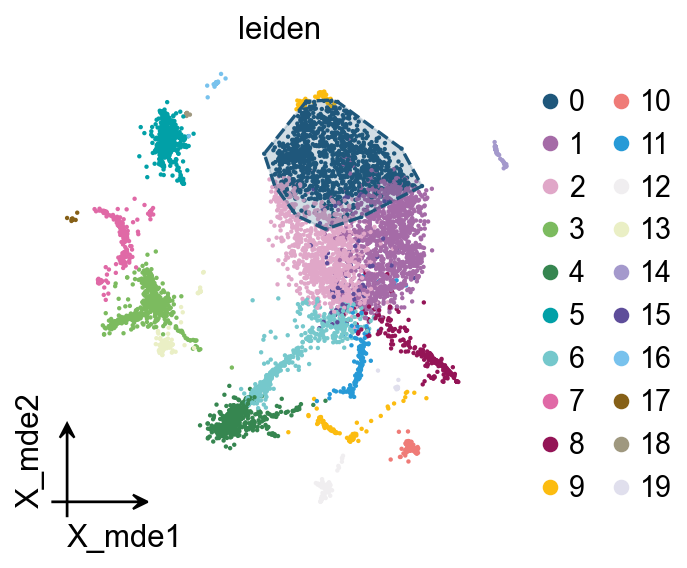
We also provide a boundary visualisation function ov.utils.plot_ConvexHull to visualise specific clusters.
Arguments:
color: if None will use the color of clusters
alpha: default is 0.2
import matplotlib.pyplot as plt
fig,ax=plt.subplots( figsize = (4,4))

ov.pl.embedding(adata,
                basis='X_mde',
                color=['leiden'],
                frameon='small',
                show=False,
                ax=ax)

ov.pl.ConvexHull(adata,
                basis='X_mde',
                cluster_key='leiden',
                hull_cluster='0',
                ax=ax)
leiden_colors
<Axes: title={'center': 'leiden'}, xlabel='X_mde1', ylabel='X_mde2'>
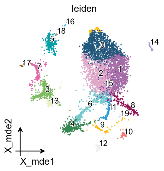
If you have too many labels, e.g. too many cell types, and you are concerned about cell overlap, then consider trying the ov.utils.gen_mpl_labels function, which improves text overlap.
In addition, we make use of the patheffects function, which makes our text have outlines
adjust_kwargs: it could be found in package
adjusttexttext_kwargs: it could be found in class
plt.texts
from matplotlib import patheffects
import matplotlib.pyplot as plt
fig, ax = plt.subplots(figsize=(4,4))

ov.pl.embedding(
    adata,
    basis='X_mde',
    color=['leiden'],
    show=False, legend_loc=None, add_outline=False,
    frameon='small',legend_fontoutline=2,ax=ax
)

ov.utils.gen_mpl_labels(
    adata,
    'leiden',
    exclude=("None",),
    basis='X_mde',
    ax=ax,
    adjust_kwargs=dict(arrowprops=dict(arrowstyle='-', color='black')),
    text_kwargs=dict(fontsize= 12 ,weight='bold',
                     path_effects=[patheffects.withStroke(linewidth=2, foreground='w')] ),
)
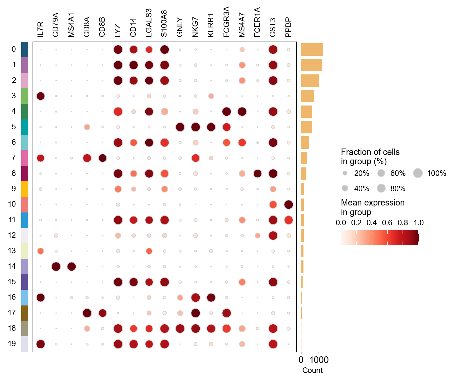
marker_genes = ['IL7R', 'CD79A', 'MS4A1', 'CD8A', 'CD8B', 'LYZ', 'CD14',
                'LGALS3', 'S100A8', 'GNLY', 'NKG7', 'KLRB1',
                'FCGR3A', 'MS4A7', 'FCER1A', 'CST3', 'PPBP']
ov.pl.dotplot(adata, marker_genes, groupby='leiden',
             standard_scale='var');
adata.write('data/pbmc_preprocessed_markers.h5ad')
Finding marker genes#
Let us compute a ranking for the highly differential genes in each cluster. For this, by default, the .raw attribute of AnnData is used in case it has been initialized before. The simplest and fastest method to do so is the t-test.
%%time
ov.single.find_markers(
    adata,
    groupby='leiden',
    method='wilcoxon',#t-test
    key_added="rank_genes_groups",
    pts=True,
)
🔍 Finding marker genes | method: wilcoxon | groupby: leiden | n_groups: 20 | n_genes: 50
✅ Done | 20 groups × 50 genes | corr: benjamini-hochberg | stored in adata.uns['rank_genes_groups']
CPU times: user 10.4 s, sys: 806 ms, total: 11.2 s
Wall time: 11.2 s
ov.single.get_markers(
    adata,
    groups=['0'],
    key = "rank_genes_groups",
)
  group  rank    names     scores  logfoldchanges          pvals  \
0     0     1   S100A8  44.998802        6.590432   0.000000e+00
1     0     2   S100A9  43.323971        6.051874   0.000000e+00
2     0     3  S100A12  39.206455        5.511002   0.000000e+00
3     0     4   S100A6  35.015156        2.022107  1.322866e-268
4     0     5     VCAN  34.773167        4.803245  6.190950e-265
5     0     6      FOS  32.592533        2.474985  5.232700e-233
6     0     7    CSF3R  32.450523        3.958353  5.325109e-231
7     0     8     TSPO  31.904837        2.399369  2.287862e-223
8     0     9  ATP5F1E  28.948526        1.022710  2.928787e-184
9     0    10     NCF1  28.933880        3.356097  4.476989e-184

       pvals_adj  pct_group  pct_rest
0   0.000000e+00   1.000000  0.589580
1   0.000000e+00   1.000000  0.644012
2   0.000000e+00   0.937450  0.417729
3  5.304694e-265   1.000000  0.929705
4  2.068809e-261   0.967923  0.515241
5  1.311445e-229   0.995188  0.874961
6  1.186316e-227   0.877306  0.477916
7  4.587164e-220   0.973536  0.801400
8  5.338379e-181   0.998396  0.961897
9  7.480302e-181   0.845229  0.520995
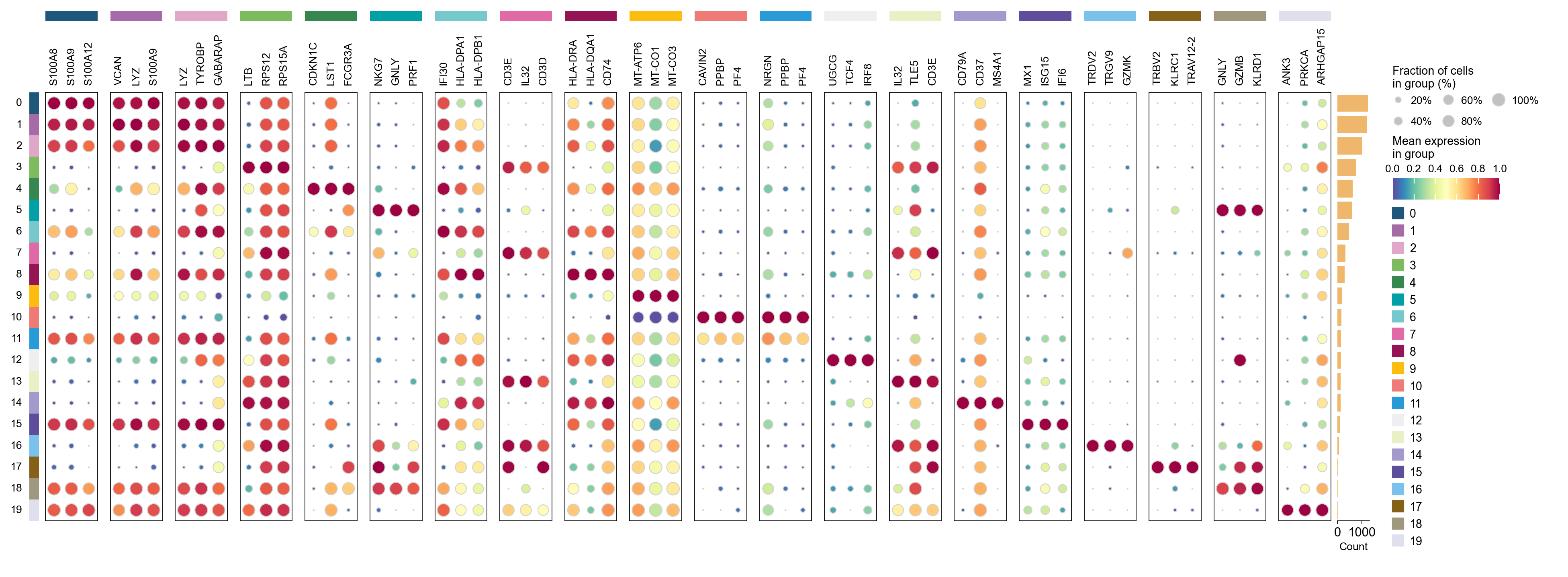
ov.pl.markers_dotplot(
    adata, groupby='leiden',
    n_genes=3,
    key="rank_genes_groups",
)
cosg is also considered to be a better algorithm for finding marker genes. Here, omicverse provides the calculation of cosg
论文: Accurate and fast cell marker gene identification with COSG
代码: genecell/COSG
%%time
ov.single.find_markers(
    adata,
    groupby='leiden',
    method='cosg',#t-test
    key_added="leiden_cosg",
    pts=True,
)
🔍 Finding marker genes | method: cosg | groupby: leiden | n_groups: 20 | n_genes: 50
**finished identifying marker genes by COSG**
✅ Done | 20 groups × 50 genes | stored in adata.uns['leiden_cosg']
CPU times: user 2.41 s, sys: 91 ms, total: 2.5 s
Wall time: 2.5 s
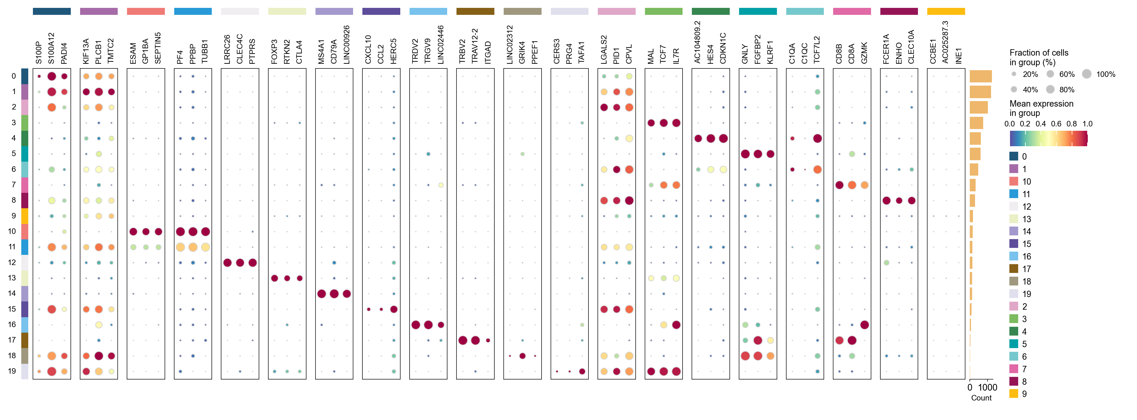
ov.pl.markers_dotplot(
    adata, groupby='leiden',
    n_genes=3,
    key="leiden_cosg",
)
ov.single.get_markers(
    adata,
    n_genes=20,
    key = "rank_genes_groups",
)
    group  rank    names     scores  logfoldchanges          pvals  \
0       0     1   S100A8  44.998802        6.590432   0.000000e+00
1       0     2   S100A9  43.323971        6.051874   0.000000e+00
2       0     3  S100A12  39.206455        5.511002   0.000000e+00
3       0     4   S100A6  35.015156        2.022107  1.322866e-268
4       0     5     VCAN  34.773167        4.803245  6.190950e-265
..    ...   ...      ...        ...             ...            ...
395    19    16      MAL   4.574203        5.732344   4.780368e-06
396    19    17   INPP4B   4.555688        6.206233   5.221436e-06
397    19    18   ABLIM1   4.504581        5.630849   6.650395e-06
398    19    19  TNFAIP8   4.450352        4.367236   8.572962e-06
399    19    20   TNRC6B   4.392069        4.240511   1.122768e-05

         pvals_adj  pct_group  pct_rest
0     0.000000e+00   1.000000  0.589580
1     0.000000e+00   1.000000  0.644012
2     0.000000e+00   0.937450  0.417729
3    5.304694e-265   1.000000  0.929705
4    2.068809e-261   0.967923  0.515241
..             ...        ...       ...
395   5.990399e-03   0.764706  0.082115
396   6.158223e-03   0.705882  0.087728
397   7.407801e-03   0.764706  0.090078
398   9.046731e-03   0.941176  0.364230
399   1.125575e-02   1.000000  0.439817

[400 rows x 9 columns]
ov.single.get_markers(
    adata,
    n_genes=5,
    key = "rank_genes_groups",
    return_type='dict'
)
{'0': ['S100A8', 'S100A9', 'S100A12', 'S100A6', 'VCAN'],
 '1': ['VCAN', 'LYZ', 'S100A9', 'FOS', 'CD14'],
 '2': ['LYZ', 'TYROBP', 'GABARAP', 'LGALS2', 'GSTP1'],
 '3': ['LTB', 'RPS12', 'RPS15A', 'RPS25', 'RPS27'],
 '4': ['CDKN1C', 'LST1', 'FCGR3A', 'SMIM25', 'MS4A7'],
 '5': ['NKG7', 'GNLY', 'PRF1', 'CTSW', 'CST7'],
 '6': ['IFI30', 'HLA-DPA1', 'HLA-DPB1', 'COTL1', 'HLA-DRA'],
 '7': ['CD3E', 'IL32', 'CD3D', 'CD8B', 'RPS3'],
 '8': ['HLA-DRA', 'HLA-DQA1', 'CD74', 'HLA-DRB1', 'HLA-DPB1'],
 '9': ['MT-ATP6', 'MT-CO1', 'MT-CO3', 'MT-CO2', 'MT-CYB'],
 '10': ['CAVIN2', 'PPBP', 'PF4', 'GNG11', 'NRGN'],
 '11': ['NRGN', 'PPBP', 'PF4', 'TUBB1', 'CAVIN2'],
 '12': ['UGCG', 'TCF4', 'IRF8', 'LILRA4', 'SERPINF1'],
 '13': ['IL32', 'TLE5', 'CD3E', 'CD3D', 'FCMR'],
 '14': ['CD79A', 'CD37', 'MS4A1', 'CD74', 'BANK1'],
 '15': ['MX1', 'ISG15', 'IFI6', 'APOBEC3A', 'TYMP'],
 '16': ['TRDV2', 'TRGV9', 'GZMK', 'CCL5', 'IL32'],
 '17': ['TRBV2', 'KLRC1', 'TRAV12-2', 'CD8A', 'CD3D'],
 '18': ['GNLY', 'GZMB', 'KLRD1', 'NKG7', 'FGFBP2'],
 '19': ['ANK3', 'PRKCA', 'ARHGAP15', 'IL7R', 'BCL11B']}