差异表达分析

bulk RNA-seq分析的一项重要任务是差异表达分析，我们可以通过omicverse来完成。对于差异表达分析，ov首先将矩阵的gene_id转换为gene_name。当数据集存在批次效应时，我们可以使用DEseq2的SizeFactors进行归一化，并使用t-test或wilcoxon检验计算基因的p值。在此，我们以featureCounts输出的矩阵为例演示此分析流程。同样的流程通常可用于分析任何RNA-seq任务。

Colab_Reproducibility：https://colab.research.google.com/drive/1q5lDfJepbtvNtc1TKz-h4wGUifTZ3i0_?usp=sharing

import omicverse as ov
import scanpy as sc
import matplotlib.pyplot as plt

ov.plot_set()

Warning: Could not read dependencies from pyproject.toml: [Errno 2] No such file or directory: '/home/groups/xiaojie/steorra/env/omicverse/lib/python3.10/site-packages/omicverse/pyproject.toml'

   ____            _     _    __                  
  / __ \____ ___  (_)___| |  / /__  _____________ 
 / / / / __ `__ \/ / ___/ | / / _ \/ ___/ ___/ _ \ 
/ /_/ / / / / / / / /__ | |/ /  __/ /  (__  )  __/ 
\____/_/ /_/ /_/_/\___/ |___/\___/_/  /____/\___/                                              

Version: 1.6.11, Tutorials: https://omicverse.readthedocs.io/

基因集下载

当我们需要转换基因id时，需要准备一个映射对文件。这里我们预处理了6个基因组gtf文件，并生成了包括T2T-CHM13、GRCh38、GRCh37、GRCm39、danRer7和danRer11的映射对。如果需要转换其他id_mapping，可以使用gtf文件生成自己的映射，将文件放在genesets目录中。

ov.utils.download_geneid_annotation_pair()

......Geneid Annotation Pair download start: pair_GRCm39
......Loading dataset from genesets/pair_GRCm39.tsv
......Geneid Annotation Pair download start: pair_T2TCHM13
......Loading dataset from genesets/pair_T2TCHM13.tsv
......Geneid Annotation Pair download start: pair_GRCh38
......Loading dataset from genesets/pair_GRCh38.tsv
......Geneid Annotation Pair download start: pair_GRCh37
......Loading dataset from genesets/pair_GRCh37.tsv
......Geneid Annotation Pair download start: pair_danRer11
......Loading dataset from genesets/pair_danRer11.tsv
......Geneid Annotation Pair download start: pair_danRer7
......Loading dataset from genesets/pair_danRer7.tsv
......Geneid Annotation Pair download finished!

注意，该数据集未经任何处理，仅由featureCounts导出，序列比对基于CRCm39基因组文件进行。

示例数据可从以下地址下载：https://raw.githubusercontent.com/Starlitnightly/omicverse/master/sample/counts.txt

data=ov.pd.read_csv('https://raw.githubusercontent.com/Starlitnightly/omicverse/master/sample/counts.txt',index_col=0,sep='\t',header=1)
#data=ov.read('data/counts.txt',index_col=0,header=1)
#replace the columns `.bam` to `` 
data.columns=[i.split('/')[-1].replace('.bam','') for i in data.columns]
data.head()

	1--1	1--2	2--1	2--2	3--1	3--2	4--1	4--2	4-3	4-4	Blank-1	Blank-2
Geneid
ENSMUSG00000102628	0	0	0	0	5	0	0	0	0	0	0	9
ENSMUSG00000100595	0	0	0	0	0	0	0	0	0	0	0	0
ENSMUSG00000097426	5	0	0	0	0	0	0	1	0	0	0	0
ENSMUSG00000104478	0	0	0	0	0	0	0	0	0	0	0	0
ENSMUSG00000104385	0	0	0	0	0	0	0	0	0	0	0	0

ID映射

我们使用之前下载的GRCm39映射对文件进行gene_id转换。

data=ov.bulk.Matrix_ID_mapping(data,'genesets/pair_GRCm39.tsv')
data.head()

	1--1	1--2	2--1	2--2	3--1	3--2	4--1	4--2	4-3	4-4	Blank-1	Blank-2
Gm37732	0	0	0	0	0	0	0	0	0	0	0	0
ENSMUSG00002075679	0	0	0	0	0	0	0	0	0	0	0	0
Mir485	0	0	0	0	0	0	0	0	0	0	0	0
Gm45619	6	1	6	3	3	9	4	2	22	3	0	17
Gm25097	0	0	0	0	0	0	0	0	0	0	0	0

使用ov进行差异表达分析

通过ov，只需提供表达矩阵，即可非常简便地进行差异表达分析。运行DEG只需：

• 通过featureCount或其他合格方法读取原始计数。

• 创建一个ov DEseq对象。

dds=ov.bulk.pyDEG(data)

我们注意到之前的gene_name映射中存在一些重复，我们将处理重复索引，仅保留表达量最高的基因。

dds.drop_duplicates_index()
print('... drop_duplicates_index success')

... drop_duplicates_index success

我们还需要去除表达矩阵的批次效应，使用DEseq2的estimateSizeFactors对矩阵进行归一化。

dds.normalize()
print('... estimateSizeFactors and normalize success')

... estimateSizeFactors and normalize success

现在我们可以从矩阵中计算差异表达基因，需要输入处理组和对照组。

ttest

treatment_groups=['4-3','4-4']
control_groups=['1--1','1--2']
result_ttest=dds.deg_analysis(treatment_groups,control_groups,method='ttest')
result_ttest.sort_values('qvalue').head()

⚙️ You are using ttest method for differential expression analysis.
⏰ Start to calculate qvalue...
✅ Differential expression analysis completed.

	pvalue	qvalue	FoldChange	MaxBaseMean	BaseMean	log2(BaseMean)	log2FC	abs(log2FC)	size	-log(pvalue)	-log(qvalue)	sig
gene_id
Uqcrh	0.000005	0.000009	1.340669	2847.780642	2485.934617	11.279573	0.422953	0.422953	0.134067	5.341574	5.050298	sig
Tdrd7	0.000016	0.000031	0.819932	570.613422	519.217650	9.020196	-0.286423	0.286423	0.081993	4.796963	4.505703	sig
Glo1-ps	0.000016	0.000032	0.538839	1718.087949	1321.875745	10.368371	-0.892074	0.892074	0.053884	4.792256	4.501011	sig
Kmt2a	0.000023	0.000045	1.203046	1337.209316	1224.344556	10.257794	0.266692	0.266692	0.120305	4.638583	4.347354	sig
5730522E02Rik	0.000028	0.000054	34.728018	7.971628	3.985814	1.994874	5.118028	5.118028	3.472802	4.560393	4.270316	sig

（可选）使用Python的edgeR

该模块是R Bioconductor edgeR包在Python中的部分移植。

result_edgepy=dds.deg_analysis(treatment_groups,control_groups,method='edgepy')
result_edgepy.sort_values('qvalue').head()

⚙️ You are using edgepy method for differential expression analysis.
⏰ Start to create DGEList...
⏰ Start to calculate qvalue...
✅ Differential expression analysis completed.

	pvalue	qvalue	FoldChange	MaxBaseMean	BaseMean	log2(BaseMean)	log2FC	abs(log2FC)	size	-log(pvalue)	-log(qvalue)	sig
gene_id
Krtap9-5	2.904895e-46	1.583284e-41	0.000473	1547.775572	774.135593	9.596442	-11.046357	11.046357	1.104636	45.536870	40.800441	sig
Krtap31-2	2.824260e-36	7.696673e-32	0.005276	2119.945065	1065.447800	10.057244	-7.566236	7.566236	0.756624	35.549095	31.113697	sig
Krtap19-4	7.394568e-34	1.343445e-29	0.007051	1801.648929	907.058833	9.825052	-7.147957	7.147957	0.714796	33.131087	28.871780	sig
Gm4553	2.906425e-33	3.960294e-29	0.007580	1747.474564	880.242980	9.781758	-7.043576	7.043576	0.704358	32.536641	28.402273	sig
Gm10153	1.665008e-29	1.512493e-25	0.000884	267.271967	133.635984	7.062165	-10.144441	10.144441	1.014444	28.778584	24.820307	sig

（可选）limma

该模块是R Bioconductor limma包在Python中的部分移植。

result_limma=dds.deg_analysis(treatment_groups,control_groups,method='limma')
result_limma.sort_values('qvalue').head()

⚙️ You are using limma method for differential expression analysis.
⏰ Start to create DGEList...
⏰ Start to adjust pvalue...
✅ Differential expression analysis completed.

	pvalue	qvalue	FoldChange	MaxBaseMean	BaseMean	log2(BaseMean)	log2FC	abs(log2FC)	size	sig	-log(pvalue)	-log(qvalue)	F	t
gene_id
Gm5853	0.000011	0.007723	5.216002	0.996454	0.498227	-1.005126	2.382945	2.382945	0.238294	sig	4.951007	2.112206	31871.910979	178.527060
Gm14409	0.000011	0.007723	5.216002	0.996454	0.498227	-1.005126	2.382945	2.382945	0.238294	sig	4.951007	2.112206	31871.910979	178.527060
Tdrd7	0.000005	0.007723	0.819932	570.613422	519.217650	9.020196	-0.286423	0.286423	0.028642	sig	5.330687	2.112206	69832.580356	-264.258548
Myl10	0.000009	0.007723	13.648007	2.989361	1.494680	0.579837	3.770618	3.770618	0.377062	sig	5.052672	2.112206	39320.908935	198.295005
5730522E02Rik	0.000009	0.007723	34.728018	7.971628	3.985814	1.994874	5.118028	5.118028	0.511803	sig	5.064980	2.112206	40333.534198	200.832105

重要的一点是，我们在处理DEG时不过滤低表达基因，在未来版本中将考虑内置相应的处理流程。

print(dds.result.shape)
dds.result=dds.result.loc[dds.result['log2(BaseMean)']>1]
print(dds.result.shape)

(54504, 14)
(21279, 14)

我们还需要设置Foldchange的阈值，我们准备了一个名为foldchange_set的方法来完成此操作。该函数根据log2FC分布自动计算合适的阈值，但您也可以手动输入。

# -1 means automatically calculates
dds.foldchange_set(fc_threshold=-1,
                   pval_threshold=0.05,
                   logp_max=6)

... Fold change threshold: 1.569942639522294

可视化DEG结果和特定基因

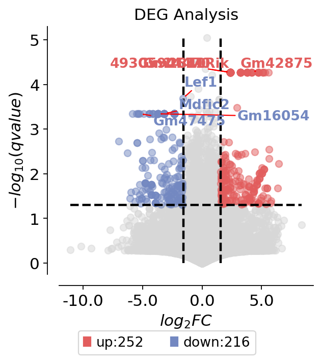
为了可视化DEG结果，我们使用plot_volcano函数。该函数可以可视化感兴趣的基因或高差异表达基因。需要输入的参数包括：

• title：火山图的标题

• figsize：图形大小

• plot_genes：您感兴趣的基因

• plot_genes_num：如果没有感兴趣的基因，可以自动绘制

dds.plot_volcano(title='DEG Analysis',figsize=(4,4),
                 plot_genes_num=8,plot_genes_fontsize=12,)

<AxesSubplot: title={'center': 'DEG Analysis'}, xlabel='$log_{2}FC$', ylabel='$-log_{10}(qvalue)$'>

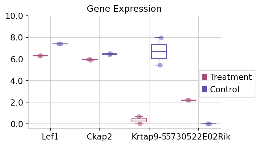
要可视化特定基因，只需使用dds.plot_boxplot函数即可。

dds.plot_boxplot(genes=['Ckap2','Lef1','Krtap9-5','5730522E02Rik'],treatment_groups=treatment_groups,
                control_groups=control_groups,figsize=(5,3),fontsize=12,
                 legend_bbox=(1.2,0.55))

(<Figure size 400x240 with 1 Axes>,
 <AxesSubplot: title={'center': 'Gene Expression'}>)

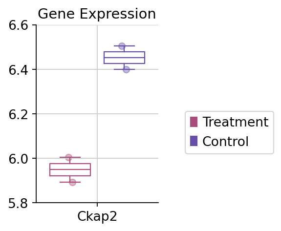
fig,ax=dds.plot_boxplot(genes=['Ckap2'],treatment_groups=treatment_groups,
                control_groups=control_groups,figsize=(2,3),fontsize=12,
                 legend_bbox=(2,0.55))
#convert the ytickbels
ax.set_yticklabels([round(float(i.get_text()),2) for i in ax.get_yticklabels()])

[Text(0, 5.800000000000001, '5.8'),
 Text(0, 6.000000000000001, '6.0'),
 Text(0, 6.200000000000001, '6.2'),
 Text(0, 6.4, '6.4'),
 Text(0, 6.6000000000000005, '6.6')]

使用ov进行通路富集分析

这里我们使用gseapy包，其中包含GSEA分析和富集分析。我们优化了该包的输出，并提供了一些更美观的图形绘制函数。

同样地，我们需要先下载通路/基因集。我们之前准备了五个基因集，可以使用ov.utils.download_pathway_database()自动下载。此外，您也可以从enrichr下载感兴趣的通路：https://maayanlab.cloud/Enrichr/#libraries

ov.utils.download_pathway_database()

......Pathway Geneset download start: GO_Biological_Process_2021
......Loading dataset from genesets/GO_Biological_Process_2021.txt
......Pathway Geneset download start: GO_Cellular_Component_2021
......Loading dataset from genesets/GO_Cellular_Component_2021.txt
......Pathway Geneset download start: GO_Molecular_Function_2021
......Loading dataset from genesets/GO_Molecular_Function_2021.txt
......Pathway Geneset download start: WikiPathway_2021_Human
......Loading dataset from genesets/WikiPathway_2021_Human.txt
......Pathway Geneset download start: WikiPathways_2019_Mouse
......Loading dataset from genesets/WikiPathways_2019_Mouse.txt
......Pathway Geneset download start: Reactome_2022
......Loading dataset from genesets/Reactome_2022.txt
......Pathway Geneset download finished!

pathway_dict=ov.utils.geneset_prepare('genesets/WikiPathways_2019_Mouse.txt',organism='Mouse')

注意，我们将pvalue_type设置为auto，这是因为当富集的基因集太小时，使用adjusted pvalue无法得到正确结果。因此您可以设置adjust或raw来获取显著的基因集。

如果没有网络连接，请将background设置为RNA-seq中表达的所有基因，例如：

enr=ov.bulk.geneset_enrichment(gene_list=deg_genes,
                                pathways_dict=pathway_dict,
                                pvalue_type='auto',
                                background=dds.result.index.tolist(),
                                organism='mouse')

deg_genes=dds.result.loc[dds.result['sig']!='normal'].index.tolist()
enr=ov.bulk.geneset_enrichment(gene_list=deg_genes,
                                pathways_dict=pathway_dict,
                                pvalue_type='auto',
                                organism='mouse')

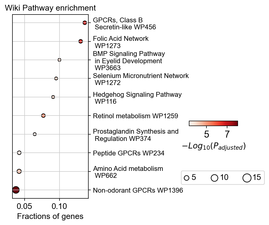
为了可视化富集结果，我们使用geneset_plot函数。

ov.bulk.geneset_plot(enr,figsize=(2,5),fig_title='Wiki Pathway enrichment',
                    cax_loc=[2, 0.45, 0.5, 0.02],
                    bbox_to_anchor_used=(-0.25, -13),node_diameter=10,
                     custom_ticks=[5,7],text_knock=3,
                    cmap='Reds')

<AxesSubplot: title={'center': 'Wiki Pathway enrichment'}, xlabel='Fractions of genes'>

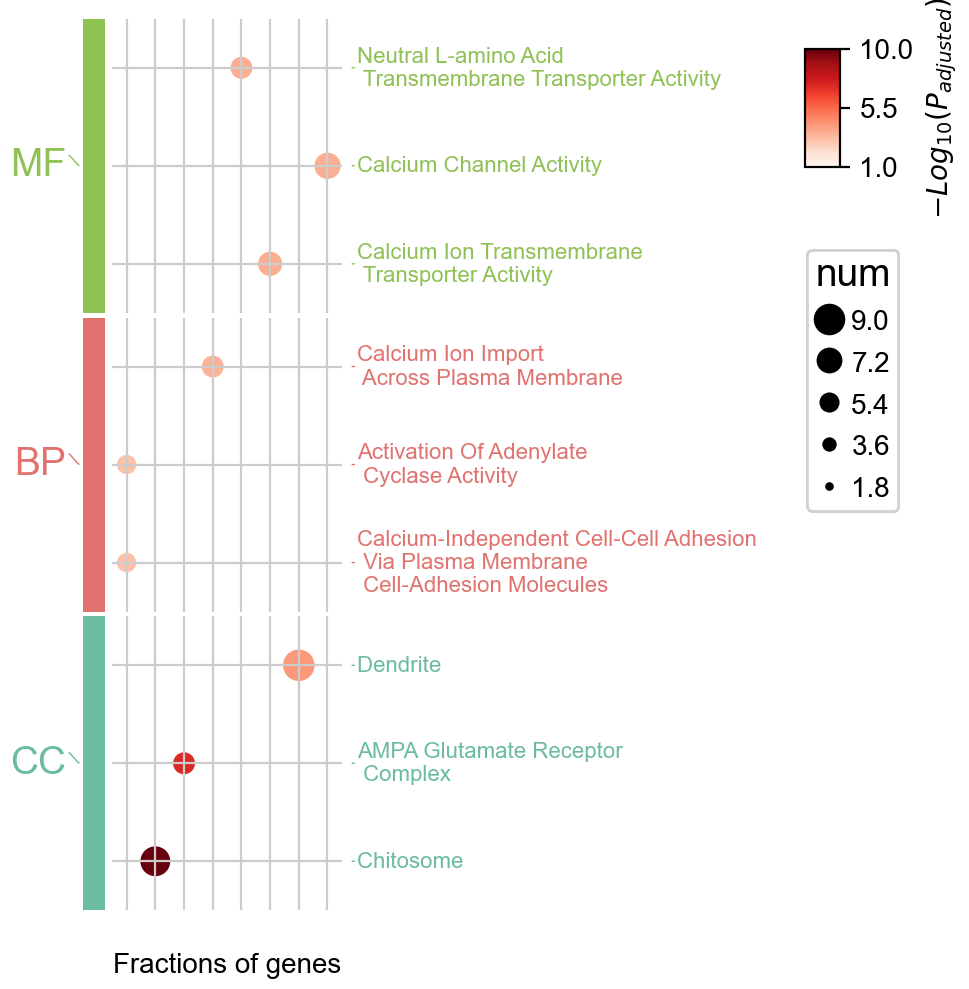
多通路富集

除了对单个数据库进行通路富集外，OmicVerse还支持同时对多个通路进行富集和可视化，这是通过pyComplexHeatmap实现的，欢迎引用！

pathway_dict=ov.utils.geneset_prepare('genesets/GO_Biological_Process_2023.txt',organism='Mouse')
enr_go_bp=ov.bulk.geneset_enrichment(gene_list=deg_genes,
                                pathways_dict=pathway_dict,
                                pvalue_type='auto',
                                organism='mouse')
pathway_dict=ov.utils.geneset_prepare('genesets/GO_Molecular_Function_2023.txt',organism='Mouse')
enr_go_mf=ov.bulk.geneset_enrichment(gene_list=deg_genes,
                                pathways_dict=pathway_dict,
                                pvalue_type='auto',
                                organism='mouse')
pathway_dict=ov.utils.geneset_prepare('genesets/GO_Cellular_Component_2023.txt',organism='Mouse')
enr_go_cc=ov.bulk.geneset_enrichment(gene_list=deg_genes,
                                pathways_dict=pathway_dict,
                                pvalue_type='auto',
                                organism='mouse')

enr_dict={'BP':enr_go_bp,
         'MF':enr_go_mf,
         'CC':enr_go_cc}
colors_dict={
    'BP':ov.pl.red_color[1],
    'MF':ov.pl.green_color[1],
    'CC':ov.pl.blue_color[1],
}
                
ov.bulk.geneset_plot_multi(enr_dict,colors_dict,num=3,
                   figsize=(2,5),
                   text_knock=3,fontsize=8,
                    cmap='Reds'
                  )

Starting plotting..
Starting calculating row orders..
Reordering rows..
Starting calculating col orders..
Reordering cols..
Plotting matrix..
Inferred max_s (max size of scatter point) is: 106.70147475919528
Collecting legends..
Plotting legends..
Estimated legend width: 9.879166666666666 mm

<Axes: ylabel='$−Log_{10}(P_{adjusted})$'>