使用DEseq2进行差异表达分析

bulk RNA-seq分析的一项重要任务是差异表达分析，我们可以通过omicverse来完成。对于差异表达分析，ov首先将矩阵的gene_id转换为gene_name。

现在我们可以使用PyDEseq2像R一样执行DESeq2分析。

Paper: PyDESeq2: a python package for bulk RNA-seq differential expression analysis

Code: owkin/PyDESeq2

Colab_Reproducibility：https://colab.research.google.com/drive/1fZS-v0zdIYkXrEoIAM1X5kPoZVfVvY5h?usp=sharing

import omicverse as ov
ov.utils.ov_plot_set()

/Users/fernandozeng/miniforge3/envs/scbasset/lib/python3.8/site-packages/phate/__init__.py

注意，该数据集未经任何处理，仅由featureCounts导出，序列比对基于CRCm39基因组文件进行。

data=ov.utils.read('https://raw.githubusercontent.com/Starlitnightly/Pyomic/master/sample/counts.txt',index_col=0,header=1)
#replace the columns `.bam` to `` 
data.columns=[i.split('/')[-1].replace('.bam','') for i in data.columns]
data.head()

	1--1	1--2	2--1	2--2	3--1	3--2	4--1	4--2	4-3	4-4	Blank-1	Blank-2
Geneid
ENSMUSG00000102628	0	0	0	0	5	0	0	0	0	0	0	9
ENSMUSG00000100595	0	0	0	0	0	0	0	0	0	0	0	0
ENSMUSG00000097426	5	0	0	0	0	0	0	1	0	0	0	0
ENSMUSG00000104478	0	0	0	0	0	0	0	0	0	0	0	0
ENSMUSG00000104385	0	0	0	0	0	0	0	0	0	0	0	0

ID映射

我们使用之前下载的GRCm39映射对文件进行gene_id转换。

ov.utils.download_geneid_annotation_pair()

data=ov.bulk.Matrix_ID_mapping(data,'genesets/pair_GRCm39.tsv')
data.head()

	1--1	1--2	2--1	2--2	3--1	3--2	4--1	4--2	4-3	4-4	Blank-1	Blank-2
Gm14845	115	116	84	86	133	170	130	105	91	127	124	99
Hdc	97	579	123	172	571	119	106	28	217	156	2	51
H2bu2	60	59	58	22	71	73	75	138	55	38	18	53
Gm6693	0	0	0	0	0	0	0	0	0	0	0	0
Rnd3	2423	2289	1996	1750	2304	2669	2952	2109	2030	2026	875	2555

使用ov进行差异表达分析

通过ov，只需提供表达矩阵，即可非常简便地进行差异表达分析。运行DEG只需：

• 通过featureCount或其他合格方法读取原始计数。

• 创建一个ov DEseq对象。

dds=ov.bulk.pyDEG(data)

我们注意到之前的gene_name映射中存在一些重复，我们将处理重复索引，仅保留表达量最高的基因。

dds.drop_duplicates_index()
print('... drop_duplicates_index success')

... drop_duplicates_index success

现在我们可以从矩阵中计算差异表达基因，需要输入处理组和对照组。

treatment_groups=['4-3','4-4']
control_groups=['1--1','1--2']
result=dds.deg_analysis(treatment_groups,control_groups,method='DEseq2')

Fitting size factors...
... done in 0.00 seconds.

Fitting dispersions...
... done in 1.59 seconds.

Fitting dispersion trend curve...
... done in 2.82 seconds.

logres_prior=1.1538905878789707, sigma_prior=0.25
Fitting MAP dispersions...
... done in 1.57 seconds.

Fitting LFCs...
... done in 1.27 seconds.

Refitting 0 outliers.

Running Wald tests...
... done in 1.33 seconds.

Log2 fold change & Wald test p-value: condition Treatment vs Control

	baseMean	log2FoldChange	lfcSE	stat	pvalue	padj
Gm14845	111.727600	-0.049168	0.470660	-0.104467	0.916799	0.975241
Hdc	258.120455	-0.809097	1.116541	-0.724646	0.468669	0.789482
H2bu2	52.656807	-0.323968	0.652995	-0.496127	0.619805	0.877166
Gm6693	0.000000	NaN	NaN	NaN	NaN	NaN
Rnd3	2180.318184	-0.183828	0.190533	-0.964809	0.334641	0.690369
...	...	...	...	...	...	...
Gm18244	0.000000	NaN	NaN	NaN	NaN	NaN
Gm50317	0.000000	NaN	NaN	NaN	NaN	NaN
Olfr516	0.000000	NaN	NaN	NaN	NaN	NaN
Gm37042	0.000000	NaN	NaN	NaN	NaN	NaN
Prelid1	3335.335908	-0.032464	0.190413	-0.170493	0.864622	0.958729

54504 rows × 6 columns

重要的一点是，我们在处理DEG时不过滤低表达基因，在未来版本中将考虑内置相应的处理流程。

print(result.shape)
result=result.loc[result['log2(BaseMean)']>1]
print(result.shape)

(54504, 14)
(23377, 14)

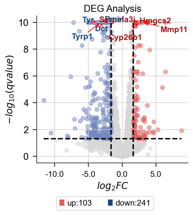
我们还需要设置Foldchange的阈值，我们准备了一个名为foldchange_set的方法来完成此操作。该函数根据log2FC分布自动计算合适的阈值，但您也可以手动输入。

# -1 means automatically calculates
dds.foldchange_set(fc_threshold=-1,
                   pval_threshold=0.05,
                   logp_max=10)

... Fold change threshold: 1.6248531033651643

可视化DEG结果和特定基因

为了可视化DEG结果，我们使用plot_volcano函数。该函数可以可视化感兴趣的基因或高差异表达基因。需要输入的参数包括：

• title：火山图的标题

• figsize：图形大小

• plot_genes：您感兴趣的基因

• plot_genes_num：如果没有感兴趣的基因，可以自动绘制

dds.plot_volcano(title='DEG Analysis',figsize=(4,4),
                 plot_genes_num=8,plot_genes_fontsize=12,)

<Axes: title={'center': 'DEG Analysis'}, xlabel='$log_{2}FC$', ylabel='$-log_{10}(qvalue)$'>

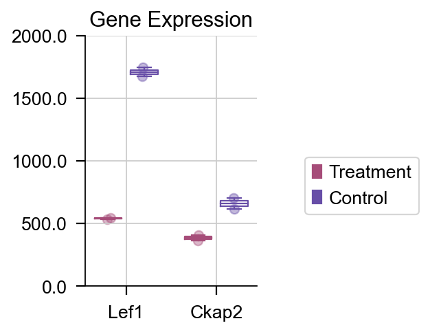
要可视化特定基因，只需使用dds.plot_boxplot函数即可。

dds.plot_boxplot(genes=['Ckap2','Lef1'],treatment_groups=treatment_groups,
                control_groups=control_groups,figsize=(2,3),fontsize=12,
                 legend_bbox=(2,0.55))

(<Figure size 160x240 with 1 Axes>,
 <Axes: title={'center': 'Gene Expression'}>)

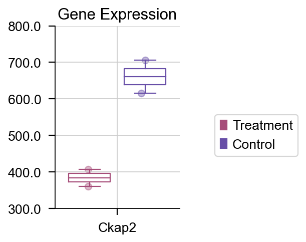
dds.plot_boxplot(genes=['Ckap2'],treatment_groups=treatment_groups,
                control_groups=control_groups,figsize=(2,3),fontsize=12,
                 legend_bbox=(2,0.55))

(<Figure size 160x240 with 1 Axes>,
 <Axes: title={'center': 'Gene Expression'}>)

使用Pyomic进行通路富集分析

这里我们使用gseapy包，其中包含GSEA分析和富集分析。我们优化了该包的输出，并提供了一些更美观的图形绘制函数。

同样地，我们需要先下载通路/基因集。我们之前准备了五个基因集，可以使用Pyomic.utils.download_pathway_database()自动下载。此外，您也可以从enrichr下载感兴趣的通路：https://maayanlab.cloud/Enrichr/#libraries

ov.utils.download_pathway_database()

......Pathway Geneset download start: GO_Biological_Process_2021
......Loading dataset from genesets/GO_Biological_Process_2021.txt
......Pathway Geneset download start: GO_Cellular_Component_2021
......Loading dataset from genesets/GO_Cellular_Component_2021.txt
......Pathway Geneset download start: GO_Molecular_Function_2021
......Loading dataset from genesets/GO_Molecular_Function_2021.txt
......Pathway Geneset download start: WikiPathway_2021_Human
......Loading dataset from genesets/WikiPathway_2021_Human.txt
......Pathway Geneset download start: WikiPathways_2019_Mouse
......Loading dataset from genesets/WikiPathways_2019_Mouse.txt
......Pathway Geneset download start: Reactome_2022
......Loading dataset from genesets/Reactome_2022.txt
......Pathway Geneset download finished!
......Other Genesets can be dowload in `https://maayanlab.cloud/Enrichr/#libraries`

pathway_dict=ov.utils.geneset_prepare('genesets/WikiPathways_2019_Mouse.txt',organism='Mouse')

要进行GSEA分析，我们首先需要对基因进行排序。使用dds.ranking2gsea可以获得按-log10(padj)排序的基因排名矩阵。

\(Metric=\frac{-log_{10}(padj)}{sign(log2FC)}\)

rnk=dds.ranking2gsea()

我们使用ov.bulk.pyGSEA构建GSEA对象以执行富集分析。

gsea_obj=ov.bulk.pyGSEA(rnk,pathway_dict)

enrich_res=gsea_obj.enrichment()

结果存储在enrich_res属性中。

gsea_obj.enrich_res.head()

	es	nes	pval	fdr	geneset_size	matched_size	genes	ledge_genes	logp	logc	num	fraction	Term	P-value
Term
Complement and Coagulation Cascades WP449	0.732116	2.140070	0.0	0.000000	62	56	Cfd;Masp1;F2r;C4b;Hc;Cfh;F7;F12;Pros1;Serping1...	Cfd;Masp1;F2r;C4b;Hc;Cfh;F7;F12;Pros1;Serping1...	9.210340	2.140070	56	0.903226	Complement and Coagulation Cascades WP449	0.000000
Matrix Metalloproteinases WP441	0.879498	2.397240	0.0	0.000000	29	27	Mmp11;Mmp14;Mmp3;Mmp12;Timp4;Timp1;Mmp28;Mmp9;...	Mmp11;Mmp14;Mmp3;Mmp12;Timp4;Timp1;Mmp28;Mmp9;...	9.210340	2.397240	27	0.931034	Matrix Metalloproteinases WP441	0.000000
TYROBP Causal Network WP3625	0.786372	2.358131	0.0	0.000000	58	57	Itgax;Itgb2;Rgs1;Gpx1;Lhfpl2;Tcirg1;Cxcl16;Cd3...	Itgax;Itgb2;Rgs1;Gpx1;Lhfpl2;Tcirg1;Cxcl16;Cd3...	9.210340	2.358131	57	0.982759	TYROBP Causal Network WP3625	0.000000
PPAR signaling pathway WP2316	0.681572	2.074737	0.0	0.003011	81	69	Hmgcs2;Pck1;Slc27a1;Scd3;Acox3;Acsbg1;Scd1;Ang...	Hmgcs2;Pck1;Slc27a1;Scd3;Acox3;Acsbg1;Scd1;Ang...	5.772960	2.074737	69	0.851852	PPAR signaling pathway WP2316	0.003011
Metapathway biotransformation WP1251	0.643937	1.991519	0.0	0.012042	141	120	Cyp26b1;Cyp2e1;Fmo2;Gpx1;Cyp4b1;Cyp11a1;Mgst2;...	Cyp26b1;Cyp2e1;Fmo2;Gpx1;Cyp4b1;Cyp11a1;Mgst2;...	4.411073	1.991519	120	0.851064	Metapathway biotransformation WP1251	0.012042

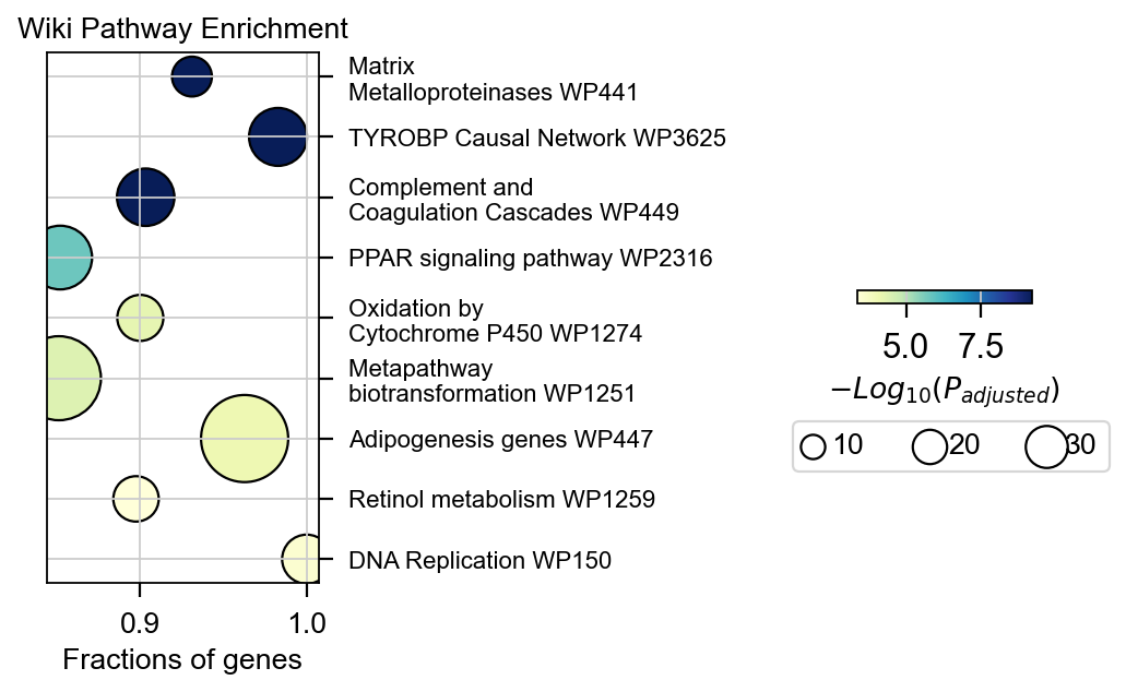
为了可视化富集结果，我们使用plot_enrichment函数。

• num：要绘制的富集条目数。默认值为10。

• node_size：定义图中节点大小的整数列表。默认为[5,10,15]。

• cax_loc：颜色条在图中的位置。默认为2。

• cax_fontsize：颜色条标签的字体大小。默认为12。

• fig_title：图的标题。默认为空字符串。

• fig_xlabel：x轴标签。默认为’Fractions of genes’。

• figsize：图的大小。默认为(2,4)。

• cmap：图中使用的颜色映射。默认为’YlGnBu’。

gsea_obj.plot_enrichment(num=10,node_size=[10,20,30],
                        cax_fontsize=12,
                        fig_title='Wiki Pathway Enrichment',fig_xlabel='Fractions of genes',
                        figsize=(2,4),cmap='YlGnBu',
                        text_knock=2,text_maxsize=30,
                        cax_loc=[2.5, 0.45, 0.5, 0.02],
                          bbox_to_anchor_used=(-0.25, -13),node_diameter=10,)

<Axes: title={'center': 'Wiki Pathway Enrichment'}, xlabel='Fractions of genes'>

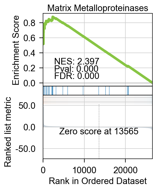
除了基础分析外，pyGSEA还帮助我们可视化带有排名和富集分数的条目。

我们可以选择要绘制的条目编号，这些编号存储在gsea_obj.enrich_res.index中，0对应Complement and Coagulation Cascades WP449，1对应Matrix Metalloproteinases WP441。

gsea_obj.enrich_res.index[:5]

Index(['Complement and Coagulation Cascades WP449',
       'Matrix Metalloproteinases WP441', 'TYROBP Causal Network WP3625',
       'PPAR signaling pathway WP2316',
       'Metapathway biotransformation WP1251'],
      dtype='object', name='Term')

我们可以设置gene_set_title来更改GSEA图的标题。

fig=gsea_obj.plot_gsea(term_num=1,
                  gene_set_title='Matrix Metalloproteinases',
                  figsize=(3,4),
                  cmap='RdBu_r',
                  title_fontsize=14,
                  title_y=0.95)