分析 Visium HD 数据

Visium HD 是 10x Genomics 推出的高分辨率空间转录组方案，用于在组织切片上直接测量基因表达。与更早期、分辨率较低的 spot 级方案相比，Visium HD 在分析上的实际变化是：我们往往要从更密集的空间单元出发，再在同一块组织的多个视图之间切换，例如规则 bin 视图和分割后的细胞视图。因此，分析重点不再只是表达矩阵本身，还包括坐标、组织图像和分割结果之间如何彼此对应。

这个教程演示了如何在 OmicVerse 中完成一条典型的 Visium HD 工作流程，同时使用 bin-level output 和 cell segmentation output 两种数据视图。整个示例覆盖四项任务：

1. 将 Visium HD 数据读入 AnnData；

2. 在组织图像上可视化基因表达；

3. 在局部区域和全切片范围内识别空间变异基因；

4. 构建低维表示，用于聚类和空间解释。

下面的代码默认你已经把 Visium HD 输出文件下载并整理到 data/visium_hd/ 目录下。

环境设置

我们先导入 OmicVerse，并启用两个 notebook 中常用的便利功能：

• ov.style(font_path='Arial')：为后续图形设置统一的绘图风格；

• %load_ext autoreload 和 %autoreload 2：在开发或调试时自动重载修改过的 Python 模块，无需反复重启内核。

import omicverse as ov
ov.style(font_path='Arial')

# 启用自动重载，便于开发和调试
%load_ext autoreload
%autoreload 2

🔬 Starting plot initialization...
Using already downloaded Arial font from: /tmp/omicverse_arial.ttf
Registered as: Arial
🧬 Detecting GPU devices…
✅ NVIDIA CUDA GPUs detected: 1
    • [CUDA 0] NVIDIA A100-SXM4-40GB
      Memory: 39.4 GB | Compute: 8.0

   ____            _     _    __                  
  / __ \____ ___  (_)___| |  / /__  _____________ 
 / / / / __ `__ \/ / ___/ | / / _ \/ ___/ ___/ _ \ 
/ /_/ / / / / / / / /__ | |/ /  __/ /  (__  )  __/ 
\____/_/ /_/ /_/_/\___/ |___/\___/_/  /____/\___/                                              

🔖 Version: 1.7.10rc1   📚 Tutorials: https://omicverse.readthedocs.io/
✅ plot_set complete.

ov.settings.cpu_gpu_mixed_init() 会以 CPU/GPU 混合模式初始化 OmicVerse。对于一部分仍然偏 CPU 的预处理步骤，以及一部分可以从 GPU 加速中受益的数值计算步骤，这种模式通常更稳妥。

ov.settings.cpu_gpu_mixed_init()

CPU-GPU mixed mode activated
Available GPU accelerators: CUDA

加载 Visium HD 数据集

Visium HD 在非常精细的空间分辨率下提供表达测量结果。实际分析时，同一份数据通常有两种视图都很有价值：

• bin-level representation：表达计数存放在规则网格上；

• cell-segmentation representation：将 bin 重新分配到分割后的细胞。

本教程会同时演示这两种视图。bin-level 对象更适合检查原始空间信号和组织图像对齐情况，而 segmentation-level 对象则更适合后续以细胞为中心的分析、空间特征发现和聚类。

在正式加载矩阵前，先查看目录结构通常会更稳妥。下面的辅助函数会打印文件树，并跳过 analysis 目录，让输出更聚焦于数据读入真正需要的文件。

这里使用的是 10x Genomics 提供的公开 Visium HD 人前列腺癌 FFPE 示例数据集，计数矩阵和组织图像可从以下页面获取： https://www.10xgenomics.com/datasets/visium-hd-cytassist-gene-expression-libraries-human-prostate-cancer-ffpe

from pathlib import Path

ov.utils.print_tree(
    Path("data/visium_hd/binned_outputs/square_016um"),
    skip_dirs={"analysis"}
)

square_016um/
    spatial/
        aligned_fiducials.jpg
        detected_tissue_image.jpg
        tissue_positions.parquet
        aligned_tissue_image.jpg
        tissue_lowres_image.png
        cytassist_image.tiff
        tissue_hires_image.png
        scalefactors_json.json
    raw_feature_bc_matrix.h5
    filtered_feature_bc_matrix/
        barcodes.tsv.gz
        features.tsv.gz
        matrix.mtx.gz
    filtered_feature_bc_matrix.h5
    raw_feature_bc_matrix/
        barcodes.tsv.gz
        features.tsv.gz
        matrix.mtx.gz

读取 bin-level 输出

第一个对象来自 square_016um 目录，这里存放的是基于规则网格分箱后的 Visium HD 数据。当你想先检查原始高分辨率空间信号，而不是立刻进入细胞层面解释时，这个视图尤其有用。

ov.io.read_visium_hd() 中有几个参数值得特别关注：

• path：所选 Visium HD 输出目录的根路径；

• data_type='bin'：告诉 OmicVerse 将输入解释为 bin-level 矩阵，而不是分割后的细胞；

• cell_matrix_h5_path 和 count_mtx_dir：分别指向 HDF5 格式和目录格式的过滤后计数矩阵；

• tissue_positions_path：提供每个 bin 的空间坐标；

• hires_image_path、lowres_image_path 和 scalefactors_path：把分子数据与组织图像关联起来，供后续绘图使用。

adata_hd = ov.io.read_visium_hd(
    path="data/visium_hd/binned_outputs/square_016um",
    data_type="bin",
    cell_matrix_h5_path="filtered_feature_bc_matrix.h5",
    count_mtx_dir='filtered_feature_bc_matrix',
    tissue_positions_path = "spatial/tissue_positions.parquet",
    # if figure and scalefactor stored in  outs/spatial
    hires_image_path="spatial/tissue_hires_image.png",
    lowres_image_path="spatial/tissue_lowres_image.png",
    scalefactors_path="spatial/scalefactors_json.json",
)

[VisiumHD][INFO] read_visium_hd entry (data_type='bin')
[VisiumHD][START] Reading bin-level data from: /scratch/users/steorra/analysis/26_omic_protocol/data/visium_hd/binned_outputs/square_016um
[VisiumHD][INFO] Sample key: square_016um
[VisiumHD][STEP] Loading count matrix (h5='filtered_feature_bc_matrix.h5', mtx='filtered_feature_bc_matrix')
[VisiumHD][STEP] Loading tissue positions: /scratch/users/steorra/analysis/26_omic_protocol/data/visium_hd/binned_outputs/square_016um/spatial/tissue_positions.parquet
[VisiumHD][STEP] Loading images and scale factors
[VisiumHD][OK] Done (n_obs=139446, n_vars=18132)

返回结果是一个标准的 AnnData 对象。此时快速检查一下观测数、基因数，以及 obs、var、obsm 和 uns 的内容，会很有帮助。

adata_hd

AnnData object with n_obs × n_vars = 139446 × 18132
    obs: 'in_tissue', 'array_row', 'array_col', 'pxl_row_in_fullres', 'pxl_col_in_fullres'
    var: 'gene_ids', 'feature_types', 'genome'
    uns: 'spatial'
    obsm: 'spatial'

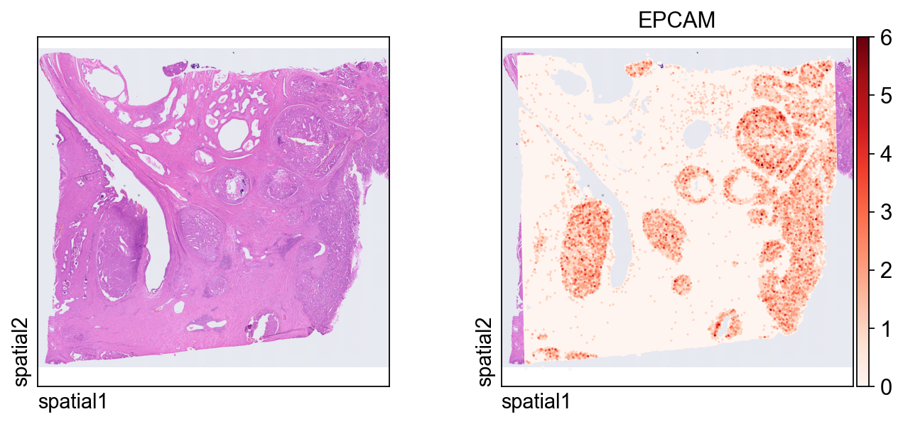
第一张图把表达信号叠加在组织图像上。

几个关键绘图参数：

• color=[None, "EPCAM"]：同时显示纯组织图像和 EPCAM 的表达；

• size：每个空间单元的点大小；

• linewidth=0：移除点边框，让高密度绘图更干净；

• cmap='Reds'：对非负表达值使用连续红色配色。

ov.pl.spatial(
    adata_hd, color=[None,"EPCAM"],
    size=3, linewidth=0,
    legend_fontsize=13, frameon=None,
    cmap='Reds'
)

读取细胞分割输出

接下来切换到 segmentation-level 输出，此时每个观测值对应的是分割后的细胞，而不再是规则 bin。这个表示通常更适合细胞层面的可视化、空间特征发现和聚类分析。

相较于 bin-level 导入，主要差别在于这里额外引入了分割文件：

• data_type='cellseg'：启用细胞分割解析模式；

• cell_segmentations_path：指向包含细胞 polygon 边界的 geojson 文件。

这两个对象实际上提供的是同一块组织的互补视图：bin-level 更适合检查原始空间结构，segmentation-level 更适合后续细胞层面的分析。

adata_seg = ov.io.read_visium_hd(
    path="data/visium_hd/segmented_outputs",
    data_type="cellseg",
    cell_matrix_h5_path="filtered_feature_cell_matrix.h5",
    cell_segmentations_path="graphclust_annotated_cell_segmentations.geojson",
    # if figure and scalefactor stored in  outs/spatial
    hires_image_path="spatial/tissue_hires_image.png",
    lowres_image_path="spatial/tissue_lowres_image.png",
    scalefactors_path="spatial/scalefactors_json.json",
)

[VisiumHD][INFO] read_visium_hd entry (data_type='cellseg')
[VisiumHD][START] Reading cell-segmentation data from: /scratch/users/steorra/analysis/26_omic_protocol/data/visium_hd/segmented_outputs
[VisiumHD][INFO] Sample key: segmented_outputs
[VisiumHD][STEP] Loading segmentation geometry: /scratch/users/steorra/analysis/26_omic_protocol/data/visium_hd/segmented_outputs/graphclust_annotated_cell_segmentations.geojson
[VisiumHD][STEP] Loading count matrix: /scratch/users/steorra/analysis/26_omic_protocol/data/visium_hd/segmented_outputs/filtered_feature_cell_matrix.h5
[VisiumHD][STEP] Loading images and scale factors
[VisiumHD][OK] Done (n_obs=227257, n_vars=18132)

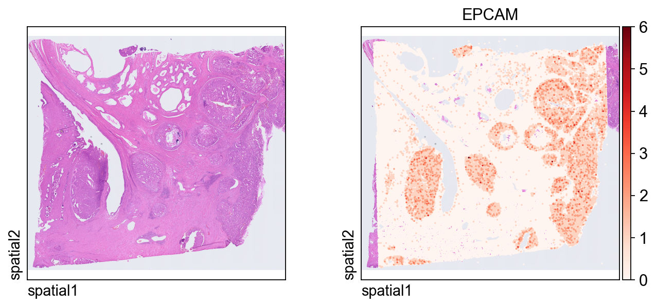
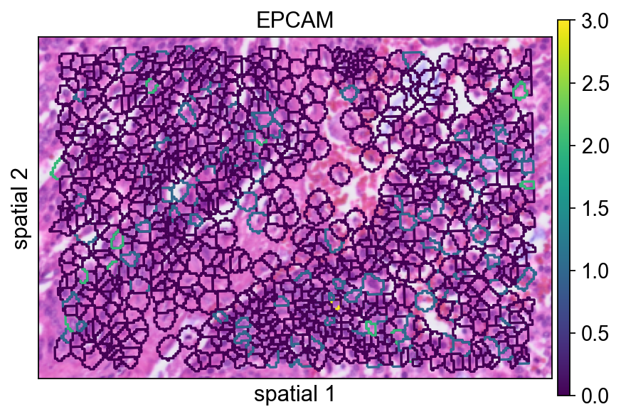
这张图在 segmentation-level 对象上展示同一个 marker EPCAM。由于每个观测现在对应一个分割细胞，因此空间模式会更容易从“细胞中心”的角度来解释。

ov.pl.spatial(
    adata_seg, color=[None,"EPCAM"],
    size=6, linewidth=0,
    legend_fontsize=13, frameon=None,
    cmap='Reds'
)

聚焦局部感兴趣区域

全切片视图适合看整体背景，但很多时候，局部窗口更方便做细节检查。下面的辅助函数会根据空间坐标对子集进行筛选。

参数说明：

• xlim 和 ylim：定义保留区域的矩形范围；

• adata.obsm["spatial"]：存储用于空间筛选的 x/y 坐标；

• obs_names_make_unique() 和 var_names_make_unique()：避免子集化后出现重复标识符。

对于高密度的 Visium HD 数据来说，这种局部放大并不只是为了好看，而是判断图像结构、分割几何和基因表达是否一致的最快方式之一。

def subset_data(adata, xlim=(24500, 26000), ylim=(5000, 6000)):
    x, y = adata.obsm["spatial"].T
    bdata = adata[(xlim[0] <= x) & (x <= xlim[1]) & (ylim[0] <= y) & (y <= ylim[1])].copy()
    bdata.obs_names_make_unique()
    bdata.var_names_make_unique()
    return bdata
bdata = subset_data(adata_seg)

接下来的几个面板会比较同一块局部分割区域的不同渲染方式。虽然这一步主要属于可视化调整，但它很适合帮助你判断最终图里应该保留多少分割边界信息。

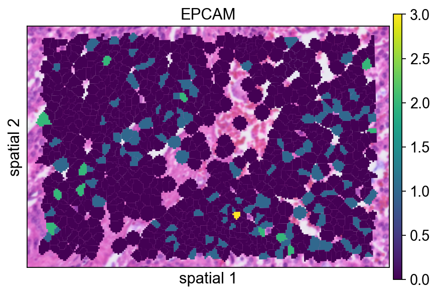
这里的分割 polygon 没有显示可见边框（edges_width=0）。这种设置更强调表达信号本身，在视野很拥挤时通常是一个不错的默认方案。

ov.pl.spatialseg(
    bdata,
    color="EPCAM",
    edges_color='white',
    edges_width=0,
    figsize=(6, 4),
    alpha_img=1,
    alpha=1,
    legend_fontsize=13,
    #cmap='Reds',
    #img_key=False,
    #alpha=1,
)

<Axes: title={'center': 'EPCAM'}, xlabel='spatial 1', ylabel='spatial 2'>

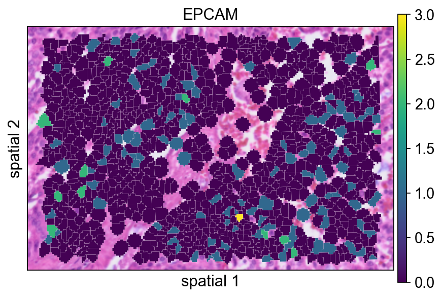
给每个 polygon 增加一条很细的边界（edges_width=0.1）有助于区分相邻细胞。当相邻 segment 的表达值比较接近时，这通常会让图更容易读。

ov.pl.spatialseg(
    bdata,
    color="EPCAM",
    edges_color='white',
    edges_width=0.1,
    figsize=(6, 4),
    alpha_img=1,
    alpha=1,
    legend_fontsize=13,
    #cmap='Reds',
    #img_key=False,
)

<Axes: title={'center': 'EPCAM'}, xlabel='spatial 1', ylabel='spatial 2'>

seg_contourpx 用像素单位控制分割轮廓的粗细。适当增大这个值能让边界更明显，尤其适合汇报图或背景组织纹理较复杂的情况。

ov.pl.spatialseg(
    bdata,
    color="EPCAM",
    edges_color='white',
    edges_width=0,
    figsize=(6, 4),
    #library_id='1',
    alpha_img=1,
    seg_contourpx=1.5,
    alpha=1,
    legend_fontsize=13,
)

<Axes: title={'center': 'EPCAM'}, xlabel='spatial 1', ylabel='spatial 2'>

识别局部区域的空间变异基因

接下来，我们在子集区域上运行 ov.space.svg()。

几个重要参数：

• mode='moranI'：使用 Moran’s I 按空间自相关对基因排序；

• n_svgs=3000：保留前 3000 个候选空间变异基因；

• n_perms=100：通过置换估计统计显著性；

• n_jobs=8：在 CPU worker 间并行计算。

bdata=ov.space.svg(
    bdata,mode='moranI',
    n_svgs=3000,
    n_perms=100,n_jobs=8,
)
bdata

Spatial neighbors: 961 cells, 5582 connections (avg 5.8 neighbors/cell).
Stored in adata.obsp['spatial_connectivities'] and adata.obsp['spatial_distances'].
Stored 18132 gene results in adata.uns['moranI'].

AnnData object with n_obs × n_vars = 961 × 18132
    obs: 'geometry'
    var: 'gene_ids', 'feature_types', 'genome', 'moranI', 'moranI_pval', 'pval_adj', 'space_variable_features', 'highly_variable'
    uns: 'spatial', 'omicverse_io', 'spatial_neighbors', 'REFERENCE_MANU', 'moranI'
    obsm: 'spatial'
    obsp: 'spatial_connectivities', 'spatial_distances'

下表可以快速查看排名靠前的基因。moranI 表示空间自相关强度，moranI_pval 记录显著性估计，space_variable_features 标记该基因是否被保留为空间特征。

bdata.var[['moranI','moranI_pval','space_variable_features']].sort_values('moranI',ascending=False)

	moranI	moranI_pval	space_variable_features
CHGA	0.422765	9.294550e-111	True
NPY	0.412106	2.276425e-105	True
PLA2G2A	0.387953	1.158365e-93	True
COL1A1	0.343667	5.067257e-74	True
KLK3	0.341580	3.733330e-73	True
...	...	...	...
SNU13	-0.033147	9.546428e-01	False
TRIOBP	-0.034662	9.617609e-01	False
SETD5	-0.036784	9.701712e-01	False
HNRNPL	-0.041451	9.833822e-01	False
TXNIP	-0.043999	9.881957e-01	False

18132 rows × 3 columns

这里以 NPY 为例展示一个具有局部空间结构的基因。使用 segmentation 渲染后，更容易判断它的信号究竟是在相邻细胞群中连续分布，还是只表现为零散点位。

ov.pl.spatialseg(
    bdata,
    color="NPY",
    edges_color='white',
    edges_width=0.1,
    figsize=(6, 4),
    alpha_img=0.8,
    alpha=1,
    legend_fontsize=13,
)

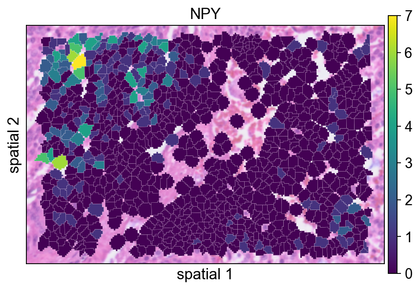
<Axes: title={'center': 'NPY'}, xlabel='spatial 1', ylabel='spatial 2'>

在归一化之前查看 X 的最大值，是一个简单但有用的 sanity check。它能帮助你快速感知当前子集对象中原始计数的大致量级。

bdata.X.max()

21.0

对局部子集做归一化和对数变换

这里的标准预处理步骤是：

• ov.pp.normalize_total(bdata)：把每个观测归一化到可比较的文库大小；

• ov.pp.log1p(bdata)：做 log(1+x) 变换，压缩动态范围。

这样处理后，空间表达图通常更容易在不同细胞之间进行比较。

ov.pp.normalize_total(bdata)
ov.pp.log1p(bdata)

🔍 Count Normalization:
   Target sum: median
   Exclude highly expressed: False

✅ Count Normalization Completed Successfully!
   ✓ Processed: 961 cells × 18,132 genes
   ✓ Runtime: 0.00s

完成归一化和 log 变换后，数值范围应明显小于原始矩阵，这说明变换已经生效。

bdata.X.max()

4.4248466

在预处理之后重新绘制 NPY，有助于判断归一化如何改变信号的视觉对比度。

ov.pl.spatialseg(
    bdata,
    color="NPY",
    edges_color='white',
    edges_width=0.1,
    figsize=(6, 4),
    alpha_img=0.8,
    alpha=1,
    legend_fontsize=13,
)

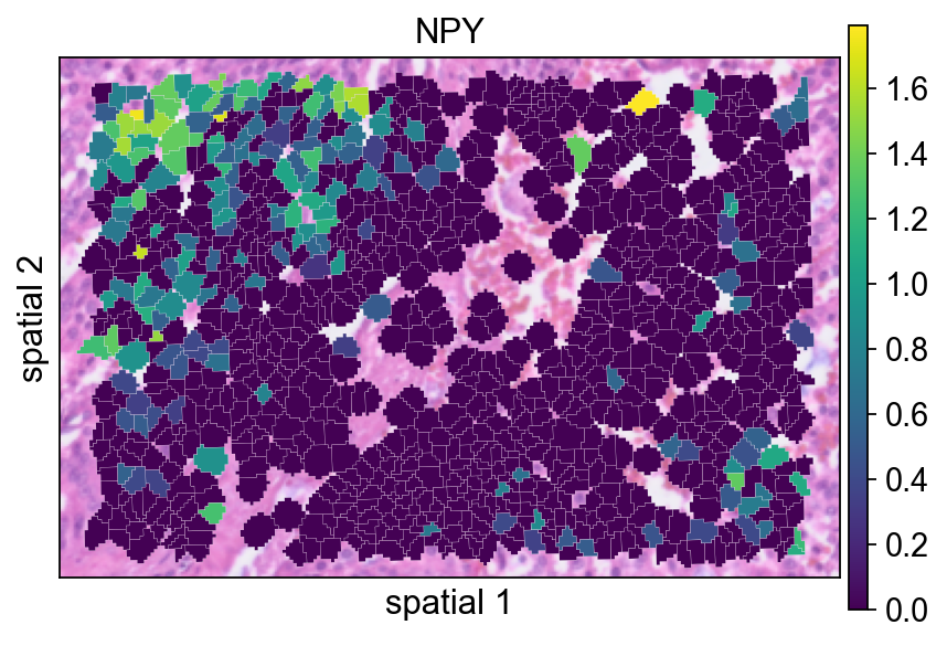
<Axes: title={'center': 'NPY'}, xlabel='spatial 1', ylabel='spatial 2'>

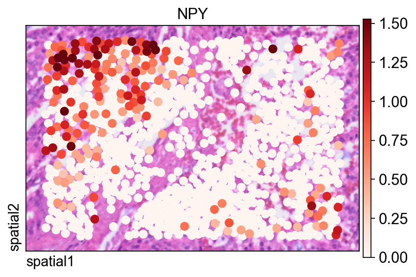
同一个基因也可以用 ov.pl.spatial() 展示，此时观测值会被渲染为点，而不是填充的分割 polygon。

这里有两个参数尤其有用：

• size=1.5：控制每个观测的点大小；

• vmax='p99.2'：把颜色上限裁剪到 99.2 百分位，减少极端值对视觉动态范围的影响。

fig, ax = ov.plt.subplots(figsize=(6, 4))
ov.pl.spatial(
    bdata, color="NPY",
    size=1.5, linewidth=0,
    legend_fontsize=13, frameon=True,
    cmap='Reds',vmax='p99.2',
    ax=ax,
)

在完整 segmentation-level 数据集上计算空间变异基因

在局部区域探索之后，我们对完整 segmentation 对象重复进行 SVG 检测。这里 notebook 使用 mode='pearsonr'，它与 Moran’s I 不同，是另一种识别空间结构的标准。

adata=ov.space.svg(
    adata_seg,mode='pearsonr',
    n_svgs=3000,
)
adata

🔍 [2026-03-08 04:48:27] Running preprocessing in 'cpu-gpu-mixed' mode...
Begin robust gene identification
    After filtration, 18109/18132 genes are kept.
    Among 18109 genes, 13307 genes are robust.
✅ Robust gene identification completed successfully.
Begin size normalization: shiftlog and HVGs selection pearson

🔍 Count Normalization:
   Target sum: 500000.0
   Exclude highly expressed: True
   Max fraction threshold: 0.2
   ⚠️ Excluding 1,410 highly-expressed genes from normalization computation
   ⚠️ Warning: 620 cells have zero counts

✅ Count Normalization Completed Successfully!
   ✓ Processed: 227,257 cells × 13,307 genes
   ✓ Runtime: 7.77s

🔍 Highly Variable Genes Selection (Experimental):
   Method: pearson_residuals
   Target genes: 3,000
   Theta (overdispersion): 100

✅ Experimental HVG Selection Completed Successfully!
   ✓ Selected: 3,000 highly variable genes out of 13,307 total (22.5%)
   ✓ Results added to AnnData object:
     • 'highly_variable': Boolean vector (adata.var)
     • 'highly_variable_rank': Float vector (adata.var)
     • 'highly_variable_nbatches': Int vector (adata.var)
     • 'highly_variable_intersection': Boolean vector (adata.var)
     • 'means': Float vector (adata.var)
     • 'variances': Float vector (adata.var)
     • 'residual_variances': Float vector (adata.var)
    Time to analyze data in cpu: 17.67 seconds.
✅ Preprocessing completed successfully.
    Added:
        'highly_variable_features', boolean vector (adata.var)
        'means', float vector (adata.var)
        'variances', float vector (adata.var)
        'residual_variances', float vector (adata.var)
        'counts', raw counts layer (adata.layers)
    End of size normalization: shiftlog and HVGs selection pearson

╭─ SUMMARY: preprocess ──────────────────────────────────────────────╮
│  Duration: 18.605s                                                 │
│  Shape:    227,257 x 18,132 -> 227,257 x 13,307                    │
│                                                                    │
│  CHANGES DETECTED                                                  │
│  ────────────────                                                  │
│  ● VAR    │ ✚ highly_variable (bool)                               │
│           │ ✚ highly_variable_features (bool)                      │
│           │ ✚ highly_variable_rank (float)                         │
│           │ ✚ means (float)                                        │
│           │ ✚ n_cells (int)                                        │
│           │ ✚ percent_cells (float)                                │
│           │ ✚ residual_variances (float)                           │
│           │ ✚ robust (bool)                                        │
│           │ ✚ variances (float)                                    │
│                                                                    │
│  ● UNS    │ ✚ REFERENCE_MANU                                       │
│           │ ✚ history_log                                          │
│           │ ✚ hvg                                                  │
│           │ ✚ log1p                                                │
│           │ ✚ status                                               │
│           │ ✚ status_args                                          │
│                                                                    │
│  ● LAYERS │ ✚ counts (sparse matrix, 227257x13307)                 │
│                                                                    │
╰────────────────────────────────────────────────────────────────────╯

AnnData object with n_obs × n_vars = 227257 × 18132
    obs: 'geometry'
    var: 'gene_ids', 'feature_types', 'genome', 'space_variable_features', 'highly_variable'
    uns: 'spatial', 'omicverse_io', 'REFERENCE_MANU'
    obsm: 'spatial'

同样地，在对完整数据集做预处理之前，先检查一下当前数值范围会更稳妥。

adata.X.max()

332.0

完整数据集会以与局部子集相同的方式完成归一化和 log 变换，这样后续降维和聚类就在可比较的尺度上进行。

ov.pp.normalize_total(adata)
ov.pp.log1p(adata)

🔍 Count Normalization:
   Target sum: median
   Exclude highly expressed: False

✅ Count Normalization Completed Successfully!
   ✓ Processed: 227,257 cells × 18,132 genes
   ✓ Runtime: 0.10s

将矩阵限制在空间变异基因上

通过 adata.raw = adata 可以保留过滤前的完整对象，方便后续参考。下一步再把矩阵限制到 adata.var.space_variable_features 标记出的基因上，从而降低噪声，并让下游分析更聚焦于空间信息更强的特征。

%%time
adata.raw = adata
adata = adata[:, adata.var.space_variable_features]
adata

CPU times: user 13 ms, sys: 70.1 ms, total: 83.1 ms
Wall time: 82.1 ms

View of AnnData object with n_obs × n_vars = 227257 × 3000
    obs: 'geometry'
    var: 'gene_ids', 'feature_types', 'genome', 'space_variable_features', 'highly_variable'
    uns: 'spatial', 'omicverse_io', 'REFERENCE_MANU', 'log1p'
    obsm: 'spatial'

构建邻接图和 UMAP 嵌入

这一单元遵循常见的流程：缩放、PCA、构图，再计算 UMAP 嵌入。

参数说明：

• PCA 中的 n_pcs=50：保留前 50 个主成分；

• n_neighbors=15：定义构图时局部邻域的大小；

• use_rep='scaled|original|X_pca'：指定 ov.pp.neighbors() 在这一工作流约定下应使用哪种处理后的表示。实际执行时，这里依赖的是上一步刚生成的 PCA 表示。

%%time
ov.pp.scale(adata)
ov.pp.pca(adata,layer='scaled',n_pcs=50)
ov.pp.neighbors(adata, n_neighbors=15, n_pcs=50,
               use_rep='scaled|original|X_pca')
ov.pp.umap(adata)

    Converting scaled data to csr_matrix format...

╭─ SUMMARY: scale ───────────────────────────────────────────────────╮
│  Duration: 29.9081s                                                │
│  Shape:    227,257 x 3,000 (Unchanged)                             │
│                                                                    │
│  CHANGES DETECTED                                                  │
│  ────────────────                                                  │
│  ● UNS    │ ✚ status                                               │
│           │ ✚ status_args                                          │
│                                                                    │
│  ● LAYERS │ ✚ scaled (sparse matrix, 227257x3000)                  │
│                                                                    │
╰────────────────────────────────────────────────────────────────────╯
🚀 Using GPU to calculate PCA...
NVIDIA CUDA GPUs detected:
📊 [CUDA 0] NVIDIA A100-SXM4-40GB
    ------------------------------ 4/40960 MiB (0.0%)
computing PCA🔍
    with n_comps=50

Using CUDA device: NVIDIA A100-SXM4-40GB
✅ Using built-in torch_pca for GPU-accelerated PCA
   🚀 Using torch_pca PCA for CUDA GPU acceleration
   🚀 torch_pca PCA backend: CUDA GPU acceleration (supports sparse matrices)
   📊 PCA input data type: SparseCSRView, shape: (227257, 3000), dtype: float64
   📊 Sparse matrix density: 100.00%
    finished✅ (2227.14s)

╭─ SUMMARY: pca ─────────────────────────────────────────────────────╮
│  Duration: 2227.5208s                                              │
│  Shape:    227,257 x 3,000 (Unchanged)                             │
│                                                                    │
│  CHANGES DETECTED                                                  │
│  ────────────────                                                  │
│  ● UNS    │ ✚ pca                                                  │
│           │ └─ params: {'zero_center': True, 'use_highly_variable': Tr...│
│           │ ✚ scaled|original|cum_sum_eigenvalues                  │
│           │ ✚ scaled|original|pca_var_ratios                       │
│                                                                    │
│  ● OBSM   │ ✚ X_pca (array, 227257x50)                             │
│           │ ✚ scaled|original|X_pca (array, 227257x50)             │
│                                                                    │
╰────────────────────────────────────────────────────────────────────╯
🚀 Using torch CPU/GPU mixed mode to calculate neighbors...
NVIDIA CUDA GPUs detected:
📊 [CUDA 0] NVIDIA A100-SXM4-40GB
    ------------------------------ 425/40960 MiB (1.0%)

🔍 K-Nearest Neighbors Graph Construction:
   Mode: cpu-gpu-mixed
   Neighbors: 15
   Method: torch
   Metric: euclidean
   Representation: scaled|original|X_pca
   PCs used: 50
   🔍 Computing neighbor distances...
   🔍 Computing connectivity matrix...
   💡 Using UMAP-style connectivity
   ✓ Graph is fully connected

✅ KNN Graph Construction Completed Successfully!
   ✓ Processed: 227,257 cells with 15 neighbors each
   ✓ Results added to AnnData object:
     • 'neighbors': Neighbors metadata (adata.uns)
     • 'distances': Distance matrix (adata.obsp)
     • 'connectivities': Connectivity matrix (adata.obsp)

╭─ SUMMARY: neighbors ───────────────────────────────────────────────╮
│  Duration: 52.9185s                                                │
│  Shape:    227,257 x 3,000 (Unchanged)                             │
│                                                                    │
│  CHANGES DETECTED                                                  │
│  ────────────────                                                  │
│  ● UNS    │ ✚ neighbors                                            │
│           │ └─ params: {'n_neighbors': 15, 'method': 'torch', 'random_...│
│                                                                    │
│  ● OBSP   │ ✚ connectivities (sparse matrix, 227257x227257)        │
│           │ ✚ distances (sparse matrix, 227257x227257)             │
│                                                                    │
╰────────────────────────────────────────────────────────────────────╯
🔍 [2026-03-08 05:27:26] Running UMAP in 'cpu-gpu-mixed' mode...
🚀 Using torch GPU to calculate UMAP...
NVIDIA CUDA GPUs detected:
📊 [CUDA 0] NVIDIA A100-SXM4-40GB
    ------------------------------ 425/40960 MiB (1.0%)

🔍 UMAP Dimensionality Reduction:
   Mode: cpu-gpu-mixed
   Method: pumap
   Components: 2
   Min distance: 0.5
{'n_neighbors': 15, 'method': 'torch', 'random_state': 0, 'metric': 'euclidean', 'use_rep': 'scaled|original|X_pca', 'n_pcs': 50}
   ⚠️ Connectivities matrix was not computed with UMAP method
   🔍 Computing UMAP parameters...
   🔍 Computing UMAP embedding (Parametric PyTorch method)...
   Using device: cuda
   Dataset: 227257 samples × 50 features
   Batch size: 512
   Learning rate: 0.001
   Training parametric UMAP model...
============================================================
🚀 Parametric UMAP Training
============================================================
📊 Device: cuda
📈 Data shape: torch.Size([227257, 50])
🔗 Building UMAP graph...
   🚀 Using PyTorch Geometric KNN (faster)

🏋️  Starting Training...
────────────────────────────────────────────────────────────
✓ New best loss: 0.2845
✓ New best loss: 0.2564
✓ New best loss: 0.2523
✓ New best loss: 0.2500
✓ New best loss: 0.2483
✓ New best loss: 0.2468
✓ New best loss: 0.2455
✓ New best loss: 0.2445
✓ New best loss: 0.2434
✓ New best loss: 0.2425
✓ New best loss: 0.2416
✓ New best loss: 0.2409
✓ New best loss: 0.2402
✓ New best loss: 0.2396
✓ New best loss: 0.2389
✓ New best loss: 0.2386
✓ New best loss: 0.2380
✓ New best loss: 0.2375
✓ New best loss: 0.2369
✓ New best loss: 0.2366

────────────────────────────────────────────────────────────
✅ Training Completed!
📉 Final best loss: 0.2366
============================================================

   💡 Using Parametric UMAP (PyTorch) on cuda

✅ UMAP Dimensionality Reduction Completed Successfully!
   ✓ Embedding shape: 227,257 cells × 2 dimensions
   ✓ Results added to AnnData object:
     • 'X_umap': UMAP coordinates (adata.obsm)
     • 'umap': UMAP parameters (adata.uns)
✅ UMAP completed successfully.

╭─ SUMMARY: umap ────────────────────────────────────────────────────╮
│  Duration: 142.413s                                                │
│  Shape:    227,257 x 3,000 (Unchanged)                             │
│                                                                    │
│  CHANGES DETECTED                                                  │
│  ────────────────                                                  │
│  ● UNS    │ ✚ umap                                                 │
│           │ └─ params: {'a': 0.583030019901822, 'b': 1.3341669931033755}│
│                                                                    │
│  ● OBSM   │ ✚ X_umap (array, 227257x2)                             │
│                                                                    │
╰────────────────────────────────────────────────────────────────────╯
⚙️ Using torch CPU/GPU mixed mode to calculate Leiden...
NVIDIA CUDA GPUs detected:
📊 [CUDA 0] NVIDIA A100-SXM4-40GB
    ------------------------------ 575/40960 MiB (1.4%)
Using batch size `n_batches` calculated from sqrt(n_obs): 476
Running GPU Leiden (batched)
Device: cpu
done: 54 clusters (0:04:36)

╭─ SUMMARY: leiden ──────────────────────────────────────────────────╮
│  Duration: 276.2389s                                               │
│  Shape:    227,257 x 3,000 (Unchanged)                             │
│                                                                    │
│  CHANGES DETECTED                                                  │
│  ────────────────                                                  │
│  ● OBS    │ ✚ leiden (category)                                    │
│                                                                    │
│  ● UNS    │ ✚ leiden                                               │
│           │ └─ params: {'resolution': 1.0, 'random_state': 0, 'local_i...│
│                                                                    │
╰────────────────────────────────────────────────────────────────────╯
CPU times: user 1h 49min 38s, sys: 27min 27s, total: 2h 17min 5s
Wall time: 45min 29s

Leiden 聚类会把图结构划分成多个社区。resolution 参数控制聚类粒度：值越低，簇越少且更粗；值越高，划分越细。

ov.pp.leiden(adata,resolution=0.3)

⚙️ Using torch CPU/GPU mixed mode to calculate Leiden...
NVIDIA CUDA GPUs detected:
📊 [CUDA 0] NVIDIA A100-SXM4-40GB
    ------------------------------ 575/40960 MiB (1.4%)
Using batch size `n_batches` calculated from sqrt(n_obs): 476
Running GPU Leiden (batched)
Device: cpu
done: 13 clusters (0:05:32)

╭─ SUMMARY: leiden ──────────────────────────────────────────────────╮
│  Duration: 332.9071s                                               │
│  Shape:    227,257 x 3,000 (Unchanged)                             │
│                                                                    │
│  CHANGES DETECTED                                                  │
│  ────────────────                                                  │
╰────────────────────────────────────────────────────────────────────╯

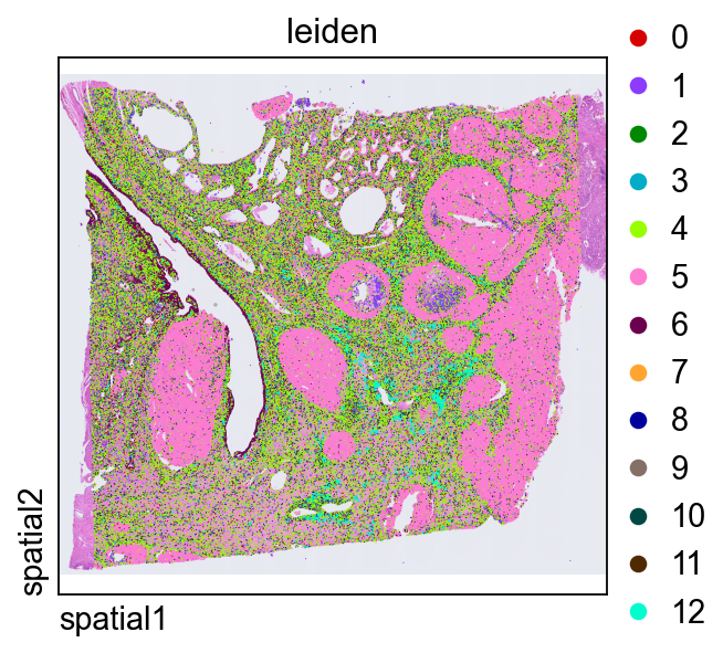
直接在组织空间中绘制 leiden，是判断转录组簇是否与连贯的解剖或组织学区域对应的快捷方式。

ov.pl.spatial(
    adata, color=["leiden"],
    size=2, linewidth=0,
    legend_fontsize=13, frameon=None,
    cmap='Reds'
)

在同一局部区域中放大查看聚类结果

最后，我们把已经聚类的数据对象裁剪到前面相同的空间窗口中。这样更方便把聚类结果与原始 marker 表达和分割边界做直接比较。

def subset_data(adata, xlim=(24500, 26000), ylim=(5000, 6000)):
    x, y = adata.obsm["spatial"].T
    bdata = adata[(xlim[0] <= x) & (x <= xlim[1]) & (ylim[0] <= y) & (y <= ylim[1])].copy()
    bdata.obs_names_make_unique()
    bdata.var_names_make_unique()
    return bdata
cdata = subset_data(adata)

这个视图把聚类标签以部分透明的方式叠加在 segmentation polygon 上，适合检查簇与簇之间的过渡是否贴合可见的组织结构。

ov.pl.spatialseg(
    cdata,
    color="leiden",
    edges_color='white',
    edges_width=0.1,
    figsize=(6, 4),
    alpha_img=0.8,
    alpha=0.8,
    legend_fontsize=13,
    palette=ov.pl.sc_color
)

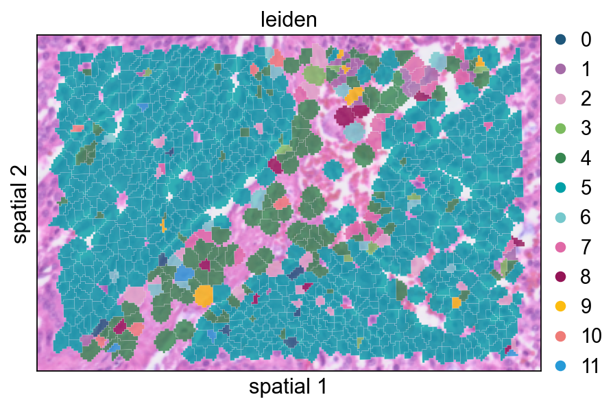
<Axes: title={'center': 'leiden'}, xlabel='spatial 1', ylabel='spatial 2'>

增大 seg_contourpx 会让 polygon 边界更锐利，这有助于观察相邻簇之间更细的分界。

ov.pl.spatialseg(
    cdata,
    color="leiden",
    edges_color='white',
    edges_width=0.1,
    figsize=(6, 4),
    alpha_img=0.8,
    alpha=1,
    legend_fontsize=13,
    palette=ov.pl.sc_color,
    seg_contourpx=1,
)

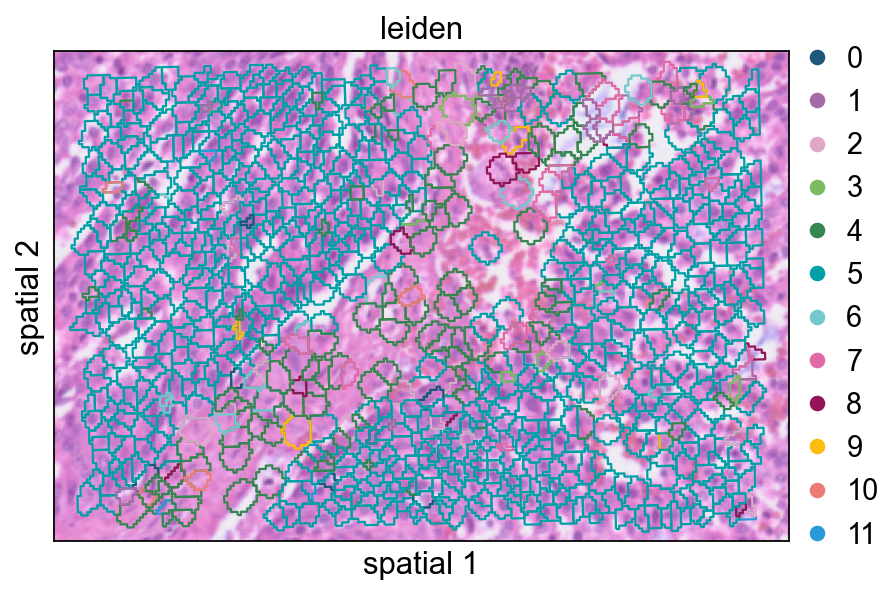
<Axes: title={'center': 'leiden'}, xlabel='spatial 1', ylabel='spatial 2'>

总结

在这个 notebook 中，我们：

• 同时导入了 bin-level 和 segmentation-level 的 Visium HD 数据；

• 比较了不同的空间可视化方式；

• 在局部和全局两个尺度上识别了空间变异基因；

• 对数据完成归一化，并把分析限制到空间特征上；

• 构建了低维表示，并对分割细胞进行聚类。

综合来看，这套流程为 OmicVerse 中的 Visium HD 分析提供了一个很实用的起点：先做图像感知的质量检查，再做空间特征筛选，最后建立细胞层面的低维表示以支撑后续解释。