FlashDeconv:通过结构保留草图实现快速空间反卷积#
这个教程展示了使用 FlashDeconv 进行空间反卷积。
import omicverse as ov
# print(f"OmicVerse version: {ov.__version__}")
🔬 Starting plot initialization...
Using already downloaded Arial font from: /tmp/omicverse_arial.ttf
Registered as: Arial
🧬 Detecting GPU devices…
✅ NVIDIA CUDA GPUs detected: 1
    • [CUDA 0] NVIDIA H100 80GB HBM3
      Memory: 79.1 GB | Compute: 9.0

   ____            _     _    __
  / __ \____ ___  (_)___| |  / /__  _____________
 / / / / __ `__ \/ / ___/ | / / _ \/ ___/ ___/ _ \
/ /_/ / / / / / / / /__ | |/ /  __/ /  (__  )  __/
\____/_/ /_/ /_/_/\___/ |___/\___/_/  /____/\___/

🔖 Version: 1.7.9rc1   📚 Tutorials: https://omicverse.readthedocs.io/
✅ plot_set complete.
第1步:加载数据#
1.1 加载 scRNA-seq 参考#
参考应包含细胞类型注释。
# 加载 scRNA-seq 参考
# 示例:人类淋巴结参考
adata_sc = ov.datasets.sc_ref_Lymph()
Subset
B_mem               13476
B_naive              8924
T_CD4+_naive         6012
B_Cycling            4765
T_CD4+_TfH           4690
T_CD8+_cytotoxic     3890
T_CD4+_TfH_GC        3653
B_activated          3575
B_GC_LZ              3298
T_CD4+               3059
T_Treg               2958
B_GC_DZ              2500
T_CD8+_CD161+        2294
T_CD8+_naive         2253
NK                   1372
B_plasma             1094
T_TfR                1065
NKT                   896
Endo                  622
ILC                   617
B_preGC               404
T_TIM3+               357
Monocytes             306
DC_pDC                226
B_IFN                 199
DC_cDC2               173
Macrophages_M1        121
Macrophages_M2        110
DC_cDC1               101
FDC                    76
B_GC_prePB             74
DC_CCR7+               42
VSMC                   40
Mast                   18
Name: count, dtype: int64
1.2 加载 空间转录组学 数据#
# 加载 spatial 数据 (示例: Visium human lymph node)adata_sp = 单细胞.数据集.visium_sge(sample_id="V1_Human_Lymph_Node")adata_sp.obs['sample'] = list(adata_sp.uns['spatial'].keys())[0]adata_sp.var_names_make_unique()print(f"Spatial 数据: {adata_sp.n_obs} 点位, {adata_sp.n_vars} 基因")
reading /scratch/users/steorra/analysis/omic_test/data/V1_Human_Lymph_Node/filtered_feature_bc_matrix.h5
 (0:00:00)
Spatial data: 4035 spots, 36601 genes
步骤 2: Run FlashDeconv DeconvolutionFlashDeconv is integrated into 该 omicverse.space.Deconvolution 类. Simply set method='FlashDeconv'.### Key 参数- sketch_dim: 维度 的 sketched space (default: 512). Higher values preserve more information.- lambda_spatial: Spatial regularization strength (default: 5000). Higher values encourage smoother spatial patterns.- n_hvg: Number 的 highly 变量 基因 到 use (default: 2000).- n_markers_per_type: Number 的 标记 基因 per 细胞类型 (default: 50).#
# Initialize 该 解卷积 objectdecov_obj = ov.space.解卷积( adata_sc=adata_sc, adata_sp=adata_sp)
# Run FlashDeconv deconvolutiondecov_obj.解卷积( 方法='FlashDeconv', celltype_key_sc='Subset', # Column containing 细胞类型 annotations flashdeconv_kwargs={ 'sketch_dim': 512, # Sketch 维度 'lambda_spatial': 10.0, # Spatial regularization 'n_hvg': 3000, # Number 的 高可变基因 'n_markers_per_type': 50, # Markers per 细胞类型 })
Running FlashDeconv with parameters: {'sketch_dim': 512, 'lambda_spatial': 10.0, 'n_hvg': 3000, 'n_markers_per_type': 50}
✓ FlashDeconv deconvolution is done
The deconvolution result is saved in self.adata_cell2location
Cell type proportions are also stored in self.adata_sp.obsm['flashdeconv']
Access ResultsResults are stored 在 multiple locations 对于 compatibility:- decov_obj.adata_cell2location: AnnData 使用 细胞类型 proportions 作为 X 矩阵- decov_obj.adata_sp.obsm['flashdeconv']: 数据框 的 proportions- decov_obj.adata_sp.obs['flashdeconv_dominant']: Dominant 细胞类型 per 点位#
# View 该 result objectdecov_obj.adata_cell2location
AnnData object with n_obs × n_vars = 4035 × 34
    obs: 'in_tissue', 'array_row', 'array_col', 'sample', 'flashdeconv_B_Cycling', 'flashdeconv_B_GC_DZ', 'flashdeconv_B_GC_LZ', 'flashdeconv_B_GC_prePB', 'flashdeconv_B_IFN', 'flashdeconv_B_activated', 'flashdeconv_B_mem', 'flashdeconv_B_naive', 'flashdeconv_B_plasma', 'flashdeconv_B_preGC', 'flashdeconv_DC_CCR7+', 'flashdeconv_DC_cDC1', 'flashdeconv_DC_cDC2', 'flashdeconv_DC_pDC', 'flashdeconv_Endo', 'flashdeconv_FDC', 'flashdeconv_ILC', 'flashdeconv_Macrophages_M1', 'flashdeconv_Macrophages_M2', 'flashdeconv_Mast', 'flashdeconv_Monocytes', 'flashdeconv_NK', 'flashdeconv_NKT', 'flashdeconv_T_CD4+', 'flashdeconv_T_CD4+_TfH', 'flashdeconv_T_CD4+_TfH_GC', 'flashdeconv_T_CD4+_naive', 'flashdeconv_T_CD8+_CD161+', 'flashdeconv_T_CD8+_cytotoxic', 'flashdeconv_T_CD8+_naive', 'flashdeconv_T_TIM3+', 'flashdeconv_T_TfR', 'flashdeconv_T_Treg', 'flashdeconv_VSMC', 'flashdeconv_dominant'
    uns: 'spatial', 'flashdeconv_params'
    obsm: 'spatial', 'flashdeconv'
# View 细胞类型 proportionsdecov_obj.adata_sp.obsm['FlashDeconv'].head()
| B_Cycling | B_GC_DZ | B_GC_LZ | B_GC_prePB | B_IFN | B_activated | B_mem | B_naive | B_plasma | B_preGC | ... | T_CD4+_TfH | T_CD4+_TfH_GC | T_CD4+_naive | T_CD8+_CD161+ | T_CD8+_cytotoxic | T_CD8+_naive | T_TIM3+ | T_TfR | T_Treg | VSMC | |
|---|---|---|---|---|---|---|---|---|---|---|---|---|---|---|---|---|---|---|---|---|---|
| AAACAAGTATCTCCCA-1 | 0.000000 | 0.142163 | 0.0 | 0.0 | 0.000000 | 0.0 | 0.0 | 0.085327 | 0.390464 | 0.0 | ... | 0.0 | 0.000000 | 0.000000 | 0.0 | 0.0 | 0.000000 | 0.000000 | 0.00000 | 0.0 | 0.040701 |
| AAACAATCTACTAGCA-1 | 0.000000 | 0.163051 | 0.0 | 0.0 | 0.000000 | 0.0 | 0.0 | 0.000000 | 0.116814 | 0.0 | ... | 0.0 | 0.049438 | 0.176642 | 0.0 | 0.0 | 0.005135 | 0.000000 | 0.15238 | 0.0 | 0.026961 |
| AAACACCAATAACTGC-1 | 0.016557 | 0.130161 | 0.0 | 0.0 | 0.000000 | 0.0 | 0.0 | 0.046586 | 0.232831 | 0.0 | ... | 0.0 | 0.000000 | 0.000000 | 0.0 | 0.0 | 0.000000 | 0.013086 | 0.00000 | 0.0 | 0.054721 |
| AAACAGAGCGACTCCT-1 | 0.000000 | 0.172508 | 0.0 | 0.0 | 0.225865 | 0.0 | 0.0 | 0.000000 | 0.078707 | 0.0 | ... | 0.0 | 0.000000 | 0.000000 | 0.0 | 0.0 | 0.000000 | 0.126967 | 0.00000 | 0.0 | 0.000000 |
| AAACAGCTTTCAGAAG-1 | 0.000000 | 0.150919 | 0.0 | 0.0 | 0.000000 | 0.0 | 0.0 | 0.403057 | 0.133602 | 0.0 | ... | 0.0 | 0.000000 | 0.000000 | 0.0 | 0.0 | 0.000000 | 0.000000 | 0.00000 | 0.0 | 0.000000 |
5 rows × 34 columns
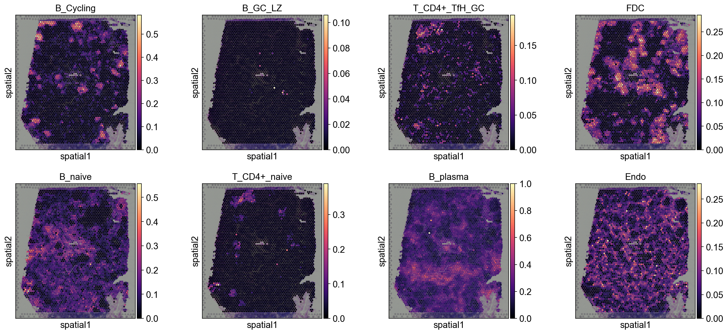
步骤 3: 可视化### 3.1 Spatial 热图 的 细胞类型 proportions#
# 选择 细胞类型 到 visualizeannotation_list=['B_Cycling', 'B_GC_LZ', 'T_CD4+_TfH_GC', 'FDC', 'B_naive', 'T_CD4+_naive', 'B_plasma', 'Endo']# 绘制 spatial distributionsc.pl.spatial( decov_obj.adata_cell2location, cmap='magma', 颜色=annotation_list, ncols=4, 大小=1.3, img_key='hires',)
3.2 Dominant 细胞类型 可视化#
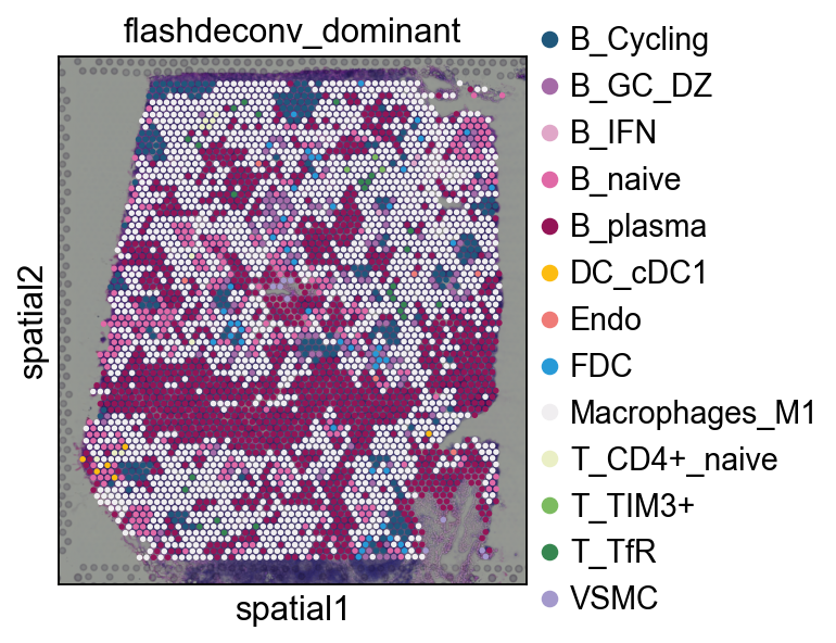
# 绘制 dominant 细胞类型 per spotsc.pl.spatial( decov_obj.adata_sp, 颜色='flashdeconv_dominant', 大小=1.3, img_key='hires',)
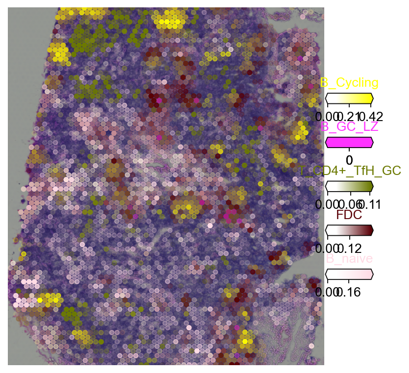
3.3 Multi-target overlay#
import matplotlib as mpl# 创建 颜色 dictionary 从 referenceif 'Subset_colors' 在 adata_sc.uns: color_dict = dict(zip( adata_sc.obs['Subset'].cat.categories, adata_sc.uns['Subset_colors'] ))否则: color_dict = Noneclust_labels = annotation_list[:5]使用 mpl.rc_context({'图.figsize': (6, 6), '轴.grid': False}): fig = ov.pl.plot_spatial( adata=decov_obj.adata_cell2location, 颜色=clust_labels, 标签=clust_labels, show_img=True, style='fast', max_color_quantile=0.992, circle_diameter=4, colorbar_position='right', palette=color_dict )
3.4 Pie chart 可视化 (cropped region)#
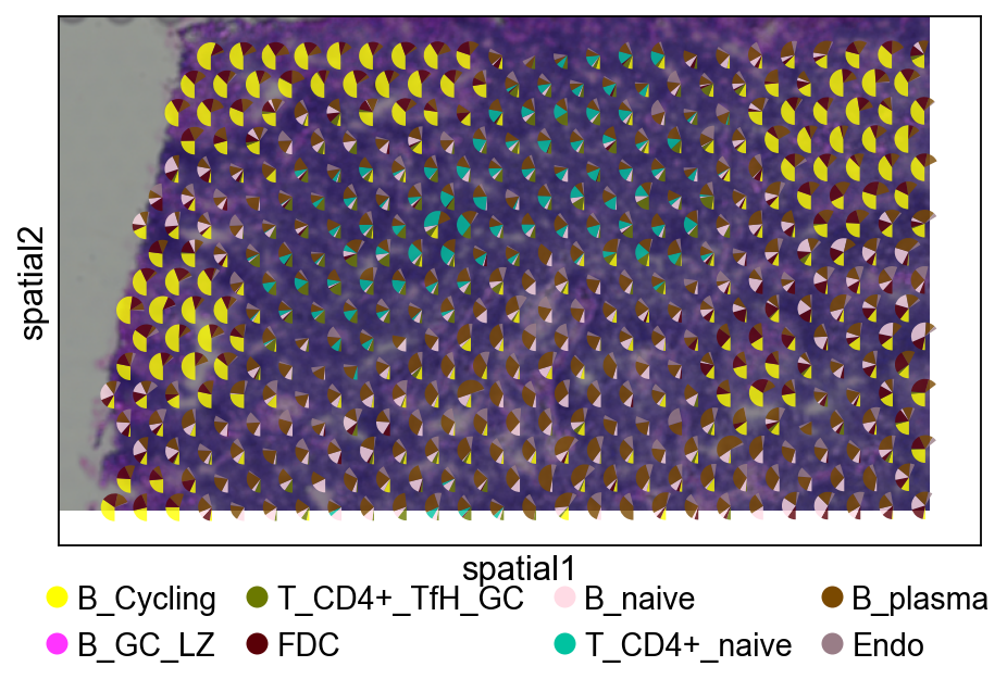
# Crop a region 的 interestadata_cropped = ov.space.crop_space_visium( decov_obj.adata_cell2location, crop_loc=(0, 0), crop_area=(500, 1000), library_id=list(decov_obj.adata_cell2location.uns['spatial'].keys())[0], 缩放=1)# 绘制 使用 pie chartsfig, ax = plt.subplots(figsize=(8, 4))单细胞.pl.spatial( adata_cropped, basis='spatial', 颜色=None, 大小=1.3, img_key='hires', ax=ax, 显示=False)ov.pl.add_pie2spatial( adata_cropped, img_key='hires', cell_type_columns=annotation_list, ax=ax, colors=color_dict, pie_radius=10, remainder='gap', legend_loc=(0.5, -0.25), ncols=4, alpha=0.8)plt.显示()
Adding image layer `image`