空间集成和聚类#
STAligner 设计用于空间转录组学数据的对齐和集成。它能够整合来自多个空间切片的数据,实现跨样本的细胞类型注释和聚类分析。
import omicverse as ov
# print(f"OmicVerse version: {ov.__version__}")
import scanpy as sc
# print(f"scanpy version: {单细胞.__version__}")
import numpy as np
# print(f"NumPy version: {np.__version__}")
from pathlib import Path

# 导入 STAligner
from omicverse.external.STAligner.STAligner import STAligner
import torch
# torch.cuda.set_device(3)
print(f'If cuda is available: {torch.cuda.is_available()}')
____            _     _    __
  / __ \____ ___  (_)___| |  / /__  _____________
 / / / / __ `__ \/ / ___/ | / / _ \/ ___/ ___/ _ \
/ /_/ / / / / / / / /__ | |/ /  __/ /  (__  )  __/
\____/_/ /_/ /_/_/\___/ |___/\___/_/  /____/\___/

Version: 1.5.4, Tutorials: https://omicverse.readthedocs.io/
预处理数据#
这里,我们使用小鼠嗅球数据,由 Stereo-seq 和 Slide-seqV2 生成两个部分。
Batch_list = []
adj_list = []
section_ids = ['Slide-seqV2_MoB', 'Stereo-seq_MoB']
print(section_ids)
path_list = [f'data/STAligner_demo/{x}/' for x in section_ids]

# 加载数据并进行标准化
for path, section_id in zip(path_list, section_ids):
    print(f'Processing {section_id}')
    adata = sc.read_h5ad(path + 'adata.h5ad')
    # 基本过滤
    sc.pp.filter_genes(adata, min_cells=3)
    sc.pp.normalize_total(adata)
    sc.pp.log1p(adata)
    adata.var['mt'] = adata.var_names.str.startswith('mt-') | adata.var_names.str.startswith('MT-')
    Batch_list.append(adata)

print('数据加载完成')
['Slide-seqV2_MoB', 'Stereo-seq_MoB']
Slide-seqV2_MoB
------Calculating spatial graph...
The graph contains 228288 edges, 20139 cells.
11.3356 neighbors per cell on average.
If you pass `n_top_genes`, all cutoffs are ignored.
extracting highly variable genes
--> added
    'highly_variable', boolean vector (adata.var)
    'highly_variable_rank', float vector (adata.var)
    'means', float vector (adata.var)
    'variances', float vector (adata.var)
    'variances_norm', float vector (adata.var)
normalizing counts per cell
    finished (0:00:00)
Stereo-seq_MoB
------Calculating spatial graph...
The graph contains 144318 edges, 19109 cells.
7.5524 neighbors per cell on average.
If you pass `n_top_genes`, all cutoffs are ignored.
extracting highly variable genes
--> added
    'highly_variable', boolean vector (adata.var)
    'highly_variable_rank', float vector (adata.var)
    'means', float vector (adata.var)
    'variances', float vector (adata.var)
    'variances_norm', float vector (adata.var)
normalizing counts per cell
    finished (0:00:00)
# # 运行 STAligner

这是运行 STAligner 对齐和集成多个空间样本的步骤。
[View of AnnData object with n_obs × n_vars = 20139 × 10000
     var: 'highly_variable', 'highly_variable_rank', 'means', 'variances', 'variances_norm'
     uns: 'Spatial_Net', 'adj', 'hvg', 'log1p'
     obsm: 'spatial',
 View of AnnData object with n_obs × n_vars = 19109 × 10000
     var: 'highly_variable', 'highly_variable_rank', 'means', 'variances', 'variances_norm'
     uns: 'Spatial_Net', 'adj', 'hvg', 'log1p'
     obsm: 'spatial']
# 初始化 STAligner
model = STAligner(
    Batch_list,
    section_ids,
    use_rep='X',
    n_components=30,
    n_neighbors=15,
    random_seed=1234
)

# 训练模型
model.train(n_epochs=300, lr=0.0002, weight_decay=0.0001, verbose=True)
adata_concat.shape: (39248, 3402)
Training STAligner modelHere, we used ov.space.pySTAligner 到 construct a STAGATE object 到 train 该 model.We are using 该 train_STAligner_subgraph 函数 从 STAligner 到 reduce GPU memory usage, each slice is considered 作为 a subgraph 对于 training.#
%%time# iter_comb is used 到 specify 该 order 的 integration. 对于 示例, (0, 1) means slice 0 will be algined 使用 slice 1 作为 参考.iter_comb = [(i, i + 1) 对于 i 在 range(len(section_ids) - 1)]# Here, 到 reduce GPU memory usage, each slice is considered 作为 a subgraph 对于 training.STAligner_obj = ov.space.pySTAligner(adata_concat, verbose=True, knn_neigh = 100, n_epochs = 600, iter_comb = iter_comb, batch_key = 'batch_name', key_added='STAligner', Batch_list = Batch_list)
STAligner(
  (conv1): GATConv(3402, 512, heads=1)
  (conv2): GATConv(512, 30, heads=1)
  (conv3): GATConv(30, 512, heads=1)
  (conv4): GATConv(512, 3402, heads=1)
)
CPU times: user 1.44 s, sys: 714 ms, total: 2.15 s
Wall time: 1.73 s
STAligner_obj.train()
Pretrain with STAGATE...
Train with STAligner...
Update spot triplets at epoch 500
We stored 该 潜在 嵌入 在 adata.obsm['STAligner'].
adata = STAligner_obj.predicted()
聚类分析 该 spaceWe can use GMM, leiden 或 louvain 到 聚类 该 space.ov.utils.cluster(adata,use_rep='STAligner',method='GMM',n_components=7,covariance_type='full', tol=1e-9, max_iter=1000, random_state=3607or sc.pp.neighbors(adata, use_rep='STAligner', random_state=666) ov.utils.cluster(adata,use_rSTAlignerGATE',method='leiden',resolution=1)#
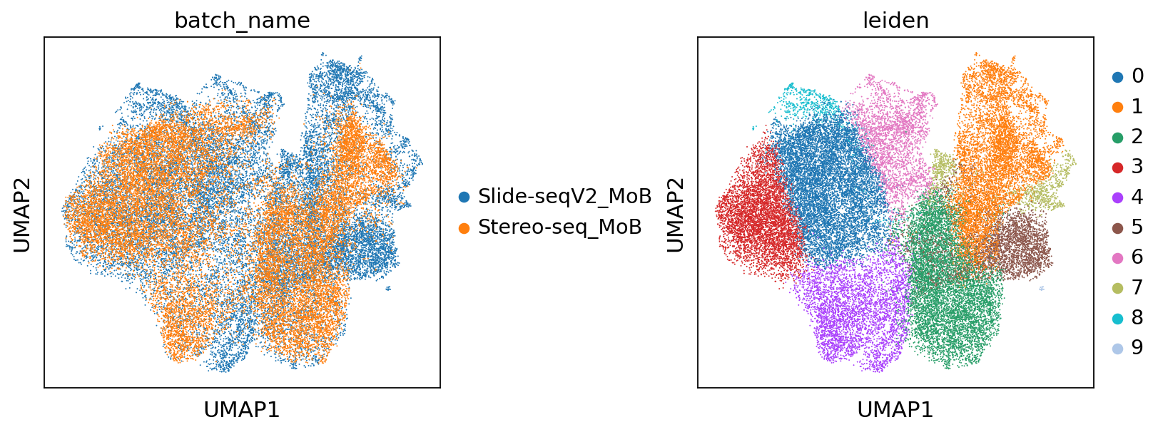
sc.pp.neighbors(adata, use_rep='STAligner', random_state=666)ov.utils.cluster(adata,use_rep='STAligner',method='leiden',resolution=0.4)sc.tl.umap(adata, random_state=666)sc.pl.umap(adata, color=['batch_name',"leiden"],wspace=0.5)
computing neighbors
    finished: added to `.uns['neighbors']`
    `.obsp['distances']`, distances for each pair of neighbors
    `.obsp['connectivities']`, weighted adjacency matrix (0:00:20)
running Leiden clustering
    finished: found 10 clusters and added
    'leiden', the cluster labels (adata.obs, categorical) (0:00:22)
computing UMAP
    finished: added
    'X_umap', UMAP coordinates (adata.obsm) (0:00:32)
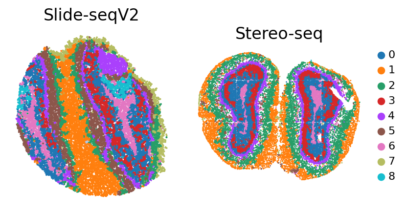
我们可以 also map 该 聚类分析 results back 到 该 original spatial coordinates 到 obtain spatially specific 聚类分析 results.
import matplotlib.pyplot as pltspot_size = 50title_size = 15fig, ax = plt.subplots(1, 2, figsize=(6, 3), gridspec_kw={'wspace': 0.05, 'hspace': 0.2})_sc_0 = sc.pl.spatial(adata[adata.obs['batch_name'] == 'Slide-seqV2_MoB'], img_key=None, color=['leiden'], title=['Slide-seqV2'], legend_fontsize=10, show=False, ax=ax[0], frameon=False, spot_size=spot_size, legend_loc=None)_sc_0[0].set_title('Slide-seqV2', size=title_size)_sc_1 = sc.pl.spatial(adata[adata.obs['batch_name'] == 'Stereo-seq_MoB'], img_key=None, color=['leiden'], title=['Stereo-seq'], legend_fontsize=10, show=False, ax=ax[1], frameon=False, spot_size=spot_size)_sc_1[0].set_title('Stereo-seq',size=title_size)_sc_1[0].invert_yaxis()plt.show()