空间聚类和降噪表达

空间聚类是空间转录组学分析的重要步骤。

import omicverse as ov
# print(f"OmicVerse version: {ov.__version__}")
import scanpy as sc
# print(f"scanpy version: {单细胞.__version__}")
import numpy as np

🔬 Starting plot initialization...
Using already downloaded Arial font from: /tmp/omicverse_arial.ttf
Registered as: Arial
🧬 Detecting GPU devices…
✅ NVIDIA CUDA GPUs detected: 1
    • [CUDA 0] NVIDIA H100 80GB HBM3
      Memory: 79.1 GB | Compute: 9.0

   ____            _     _    __                  
  / __ \____ ___  (_)___| |  / /__  _____________ 
 / / / / __ `__ \/ / ___/ | / / _ \/ ___/ ___/ _ \ 
/ /_/ / / / / / / / /__ | |/ /  __/ /  (__  )  __/ 
\____/_/ /_/ /_/_/\___/ |___/\___/_/  /____/\___/                                              

🔖 Version: 1.7.9rc1   📚 Tutorials: https://omicverse.readthedocs.io/
✅ plot_set complete.

预处理数据

数据预处理包括过滤、标准化和质量控制。

# 加载数据
adata = sc.read_h5ad('data/adata_sample.h5ad')
print(f'数据形状: {adata.shape}')

reading data/151676/151676_filtered_feature_bc_matrix.h5
 (0:00:00)

Note

We introduced 该 spatial special svg calculation module prost 在 OmicVerse versions greater than `1.6.0` 到 replace scanpy's 高可变基因, 如果 you want 到 use scanpy's 高可变基因 you can set mode=`scanpy` 在 `ov.space.svg` 或 use 该 following code.

```python#adata=ov.pp.preprocess(adata,mode='shiftlog|pearson',n_HVGs=3000,target_sum=1e4)#adata.raw = adata#adata = adata[:, adata.var.highly_variable_features]```

sc.pp.calculate_qc_metrics(adata, inplace=True)adata = adata[:,adata.var['total_counts']>100]adata=ov.space.svg(adata,mode='pearsonr',n_svgs=3000,                   target_sum=1e4,platform="visium",)adata

🔍 [2026-01-08 00:32:43] Running preprocessing in 'cpu' mode...
Begin robust gene identification
    After filtration, 10747/10747 genes are kept.
    Among 10747 genes, 10747 genes are robust.
✅ Robust gene identification completed successfully.
Begin size normalization: shiftlog and HVGs selection pearson

🔍 Count Normalization:
   Target sum: 10000.0
   Exclude highly expressed: True
   Max fraction threshold: 0.2
   ⚠️ Excluding 0 highly-expressed genes from normalization computation
   Excluded genes: []

✅ Count Normalization Completed Successfully!
   ✓ Processed: 3,460 cells × 10,747 genes
   ✓ Runtime: 0.14s

🔍 Highly Variable Genes Selection (Experimental):
   Method: pearson_residuals
   Target genes: 3,000
   Theta (overdispersion): 100

✅ Experimental HVG Selection Completed Successfully!
   ✓ Selected: 3,000 highly variable genes out of 10,747 total (27.9%)
   ✓ Results added to AnnData object:
     • 'highly_variable': Boolean vector (adata.var)
     • 'highly_variable_rank': Float vector (adata.var)
     • 'highly_variable_nbatches': Int vector (adata.var)
     • 'highly_variable_intersection': Boolean vector (adata.var)
     • 'means': Float vector (adata.var)
     • 'variances': Float vector (adata.var)
     • 'residual_variances': Float vector (adata.var)
    Time to analyze data in cpu: 1.34 seconds.
computing PCA
    with n_comps=50
    finished (0:00:01)
✅ Preprocessing completed successfully.
    Added:
        'highly_variable_features', boolean vector (adata.var)
        'means', float vector (adata.var)
        'variances', float vector (adata.var)
        'residual_variances', float vector (adata.var)
        'counts', raw counts layer (adata.layers)
    End of size normalization: shiftlog and HVGs selection pearson

AnnData object with n_obs × n_vars = 3460 × 10747
    obs: 'in_tissue', 'array_row', 'array_col', 'n_genes_by_counts', 'log1p_n_genes_by_counts', 'total_counts', 'log1p_total_counts', 'pct_counts_in_top_50_genes', 'pct_counts_in_top_100_genes', 'pct_counts_in_top_200_genes', 'pct_counts_in_top_500_genes'
    var: 'gene_ids', 'feature_types', 'genome', 'n_cells_by_counts', 'mean_counts', 'log1p_mean_counts', 'pct_dropout_by_counts', 'total_counts', 'log1p_total_counts', 'n_cells', 'percent_cells', 'robust', 'highly_variable_features', 'means', 'variances', 'residual_variances', 'highly_variable_rank', 'highly_variable', 'space_variable_features'
    uns: 'spatial', 'log1p', 'hvg', 'pca', 'status', 'status_args', 'REFERENCE_MANU'
    obsm: 'spatial', 'X_pca'
    varm: 'PCs'
    layers: 'counts'

adata.write('data/cluster_svg.h5ad',compression='gzip')

adata=ov.read('data/cluster_svg.h5ad',compression='gzip')

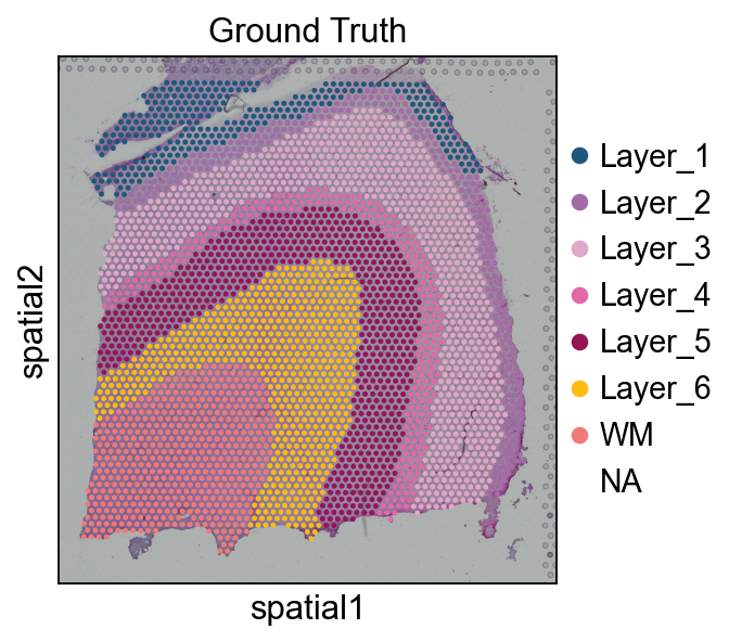
(Optional) We 读取 该 ground truth area 的 our spatial dataThis 步骤 is not mandatory 到 run, 在 该 教程, it’s just 到 demonstrate 该 accuracy 的 our 聚类分析 effect, 和 在 your own tasks, there is often no Ground_truth

# 读取 该 annotationimport Pandas 作为 pdimport osAnn_df = pd.read_csv(os.路径.join('数据/151676', '151676_truth.txt'), sep='\t', header=None, index_col=0)Ann_df.columns = ['Ground Truth']adata.obs['Ground Truth'] = Ann_df.loc[adata.obs_names, 'Ground Truth']单细胞.pl.spatial(adata, img_key="hires", 颜色=["Ground Truth"])

Method1: GraphSTGraphST was rated 作为 one 的 该 best spatial 聚类分析 algorithms 在 Nature 方法 2024.04, so we first tried 到 call GraphST 对于 spatial domain identification 在 OmicVerse.

methods_kwargs={}methods_kwargs['GraphST']={    'device':'cuda:0',    'n_pcs':30}adata=ov.space.clusters(adata,                  methods=['GraphST'],                  methods_kwargs=methods_kwargs,                  lognorm=1e4)

The GraphST method is used to embed the spatial data.
Begin to train ST data...
Optimization finished for ST data!
computing PCA
    with n_comps=30
    finished (0:00:01)
GraphST embedding has been saved in adata.obsm["GraphST_embedding"]                         and adata.obsm["graphst|original|X_pca"]
The GraphST embedding are stored in adata.obsm["GraphST_embedding"]. 
Shape: (3460, 3000)

ov.utils.cluster(adata,use_rep='graphst|original|X_pca',method='mclust',n_components=10,                 modelNames='EEV', random_state=112,                )adata.obs['mclust_GraphST'] = ov.utils.refine_label(adata, radius=50, key='mclust') adata.obs['mclust_GraphST']=adata.obs['mclust_GraphST'].astype('category')

running GaussianMixture clustering
finished: found 10 clusters and added
    'mclust', the cluster labels (adata.obs, categorical)

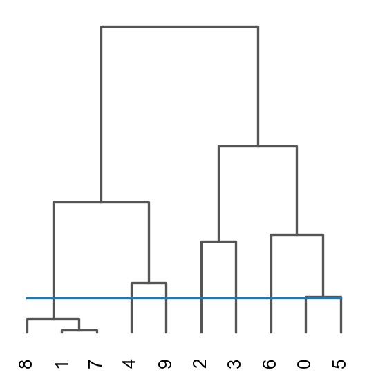
res=ov.space.merge_cluster(adata,groupby='mclust_GraphST',use_rep='graphst|original|X_pca',                  threshold=0.2,plot=True)

Storing dendrogram info using `.uns['dendrogram_mclust_GraphST']`
The merged cluster information is stored in adata.obs["mclust_GraphST_tree"].

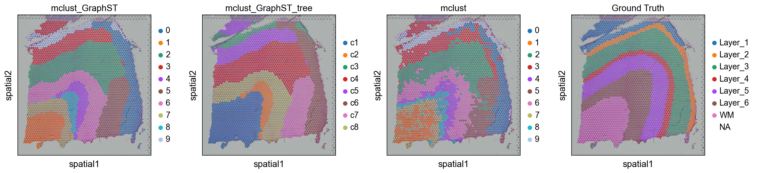
sc.pl.spatial(adata, color=['mclust_GraphST','mclust_GraphST_tree','mclust','Ground Truth'])

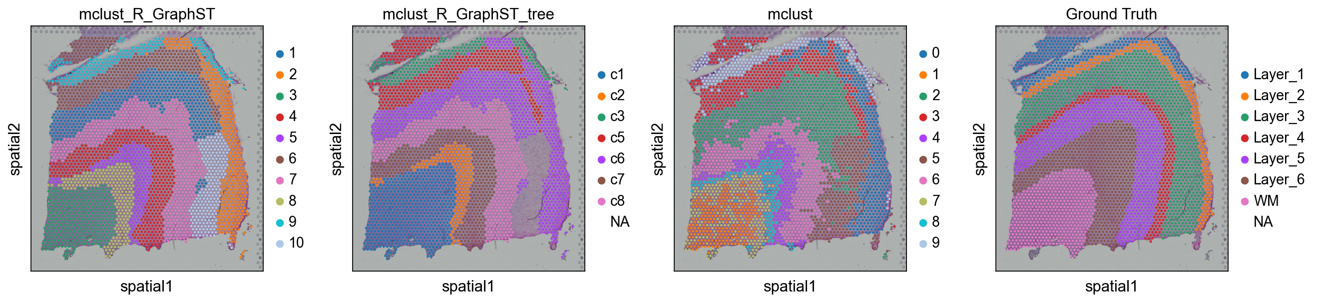
我们可以 also use mclust_R 到 聚类 该 spatial domain, but 此 方法 need 到 安装 rpy2 在 first.该 use 的 该 mclust algorithm requires 该 rpy2 package 和 该 mclust package. See https://pypi.org/project/rpy2/ 和 https://cran.r-project.org/web/packages/mclust/index.html 对于 detail.

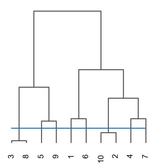
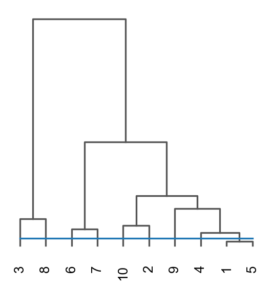
ov.utils.cluster(adata,use_rep='graphst|original|X_pca',method='mclust_R',n_components=10,                 random_state=42,                )adata.obs['mclust_R_GraphST'] = ov.utils.refine_label(adata, radius=30, key='mclust_R') adata.obs['mclust_R_GraphST']=adata.obs['mclust_R_GraphST'].astype('category')res=ov.space.merge_cluster(adata,groupby='mclust_R_GraphST',use_rep='graphst|original|X_pca',                  threshold=0.2,plot=True)

fitting ...
  |======================================================================| 100%
finished: found 10 clusters and added
    'mclust', the cluster labels (adata.obs, categorical)
Storing dendrogram info using `.uns['dendrogram_mclust_R_GraphST']`
The merged cluster information is stored in adata.obs["mclust_R_GraphST_tree"].

sc.pl.spatial(adata, color=['mclust_R_GraphST','mclust_R_GraphST_tree','mclust','Ground Truth'])

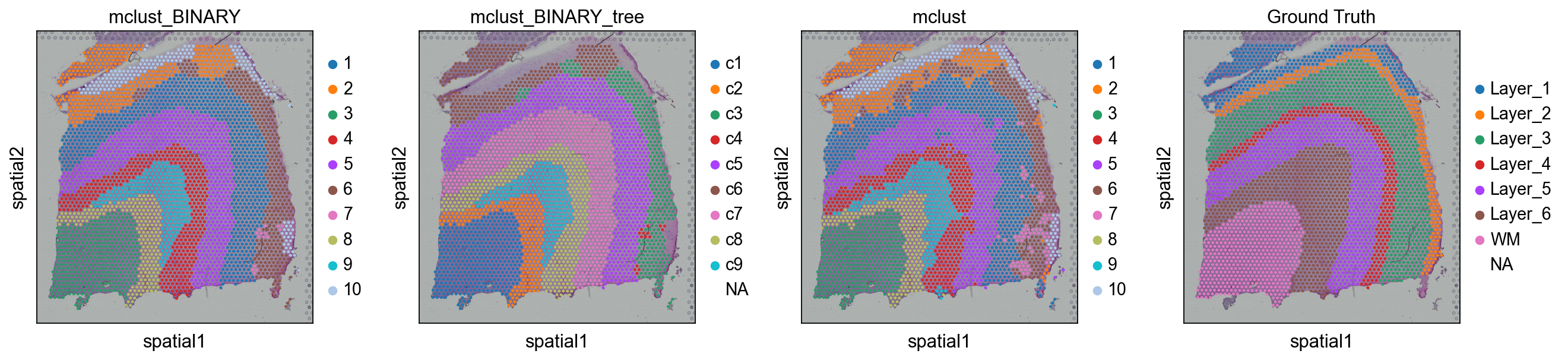
Method2: BINARYBINARY outperforms existing 方法 across various SRT 数据 types 当 using significantly less input information.如果 your 数据 is very large, 或 very 稀疏, I believe BINARY would be a great choice.

methods_kwargs={}methods_kwargs['BINARY']={    'use_method':'KNN',    'cutoff':6,    'obs_key':'BINARY_sample',    'use_list':None,    'pos_weight':10,    'device':'cuda:0',    'hidden_dims':[512, 30],    'n_epochs': 1000,    'lr':  0.001,    'key_added': 'BINARY',    'gradient_clipping': 5,    'weight_decay': 0.0001,    'verbose': True,    'random_seed':0,    'lognorm':1e4,    'n_top_genes':2000,}adata=ov.space.clusters(adata,                  methods=['BINARY'],                 methods_kwargs=methods_kwargs)

The BINARY method is used to embed the spatial data.
Recover the counts matrix from log-normalized data.
extracting highly variable genes
--> added
    'highly_variable', boolean vector (adata.var)
    'highly_variable_rank', float vector (adata.var)
    'means', float vector (adata.var)
    'variances', float vector (adata.var)
    'variances_norm', float vector (adata.var)
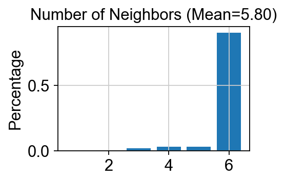
------Constructing spatial graph...------
The graph contains 20760 edges, 3460 cells.
6.0000 neighbors per cell on average.
Size of Input:  (3460, 2000)
The binary embedding are stored in adata.obsm["BINARY"]. 
Shape: (3460, 30)

如果 you want 到 use R’s mclust, you can use ov.utils.cluster.But you need 到 安装 rpy2 和 mclust 在 first.

ov.utils.cluster(adata,use_rep='BINARY',method='mclust_R',n_components=10,                 random_state=42,                )adata.obs['mclust_BINARY'] = ov.utils.refine_label(adata, radius=30, key='mclust_R') adata.obs['mclust_BINARY']=adata.obs['mclust_BINARY'].astype('category')

fitting ...
  |======================================================================| 100%

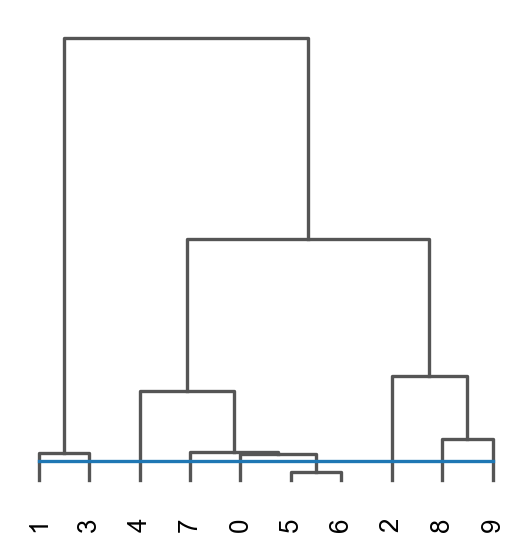
res=ov.space.merge_cluster(adata,groupby='mclust_BINARY',use_rep='BINARY',                  threshold=0.01,plot=True)

Storing dendrogram info using `.uns['dendrogram_mclust_BINARY']`
The merged cluster information is stored in adata.obs["mclust_BINARY_tree"].

sc.pl.spatial(adata, color=['mclust_BINARY','mclust_BINARY_tree','mclust','Ground Truth'])

ov.utils.cluster(adata,use_rep='BINARY',method='mclust',n_components=10,                 modelNames='EEV', random_state=42,                )adata.obs['mclustpy_BINARY'] = ov.utils.refine_label(adata, radius=30, key='mclust') adata.obs['mclustpy_BINARY']=adata.obs['mclustpy_BINARY'].astype('category')

running GaussianMixture clustering
finished: found 10 clusters and added
    'mclust', the cluster labels (adata.obs, categorical)

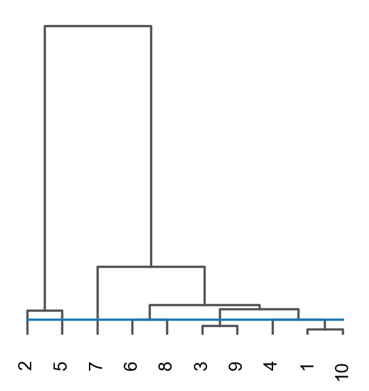
adata.obs['mclustpy_BINARY']=adata.obs['mclustpy_BINARY'].astype('category')res=ov.space.merge_cluster(adata,groupby='mclustpy_BINARY',use_rep='BINARY',                  threshold=0.013,plot=True)

Storing dendrogram info using `.uns['dendrogram_mclustpy_BINARY']`
The merged cluster information is stored in adata.obs["mclustpy_BINARY_tree"].

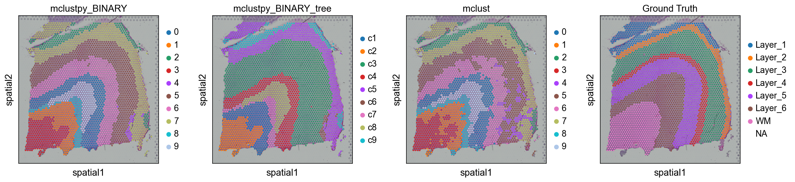
sc.pl.spatial(adata, color=['mclustpy_BINARY','mclustpy_BINARY_tree','mclust','Ground Truth'])# adata.obs['mclust_BINARY'] = ov.utils.refine_label(adata, radius=30, key='mclust') #adata.obs['mclust_BINARY']=adata.obs['mclust_BINARY'].astype('category')

Method3: STAGATESTAGATE is designed 对于 spatial 聚类分析 和 denoising expressions 的 spatial resolved transcriptomics (空间转录组) 数据.STAGATE learns 低-dimensional 潜在 嵌入 使用 both spatial information 和 基因 expressions via a graph attention auto-encoder. 该 方法 adopts an attention mechanism 在 该 middle layer 的 该 encoder 和 decoder, which adaptively learns 该 edge weights 的 spatial neighbor networks, 和 further uses them 到 update 该 点位 representation 通过 collectively aggregating information 从 its neighbors. 该 潜在 嵌入 和 该 reconstructed 表达 profiles can be used 到 downstream tasks such 作为 spatial domain identification, 可视化, spatial trajectory inference, 数据 denoising 和 3D 表达 domain extraction.Dong, Kangning, 和 Shihua Zhang. “Deciphering spatial domains 从 spatially resolved transcriptomics 使用 an adaptive graph attention auto-encoder.” Nature Communications 13.1 (2022): 1-12.Here, we used ov.space.pySTAGATE 到 construct a STAGATE object 到 train 该 model.

methods_kwargs={}methods_kwargs['STAGATE']={    'num_batch_x':3,'num_batch_y':2,    'spatial_key':['X','Y'],'rad_cutoff':200,    'num_epoch':1000,'lr':0.001,    'weight_decay':1e-4,'hidden_dims':[512, 30],    'device':'cuda:0',    # 'n_top_genes':2000,}adata=ov.space.clusters(adata,                  方法=['STAGATE'],                 methods_kwargs=methods_kwargs)

The STAGATE method is used to cluster the spatial data.
------Calculating spatial graph...
The graph contains 3060 edges, 559 cells.
5.4741 neighbors per cell on average.
------Calculating spatial graph...
The graph contains 3328 edges, 595 cells.
5.5933 neighbors per cell on average.
------Calculating spatial graph...
The graph contains 3448 edges, 613 cells.
5.6248 neighbors per cell on average.
------Calculating spatial graph...
The graph contains 3044 edges, 541 cells.
5.6266 neighbors per cell on average.
------Calculating spatial graph...
The graph contains 3128 edges, 559 cells.
5.5957 neighbors per cell on average.
------Calculating spatial graph...
The graph contains 3320 edges, 595 cells.
5.5798 neighbors per cell on average.
------Calculating spatial graph...
The graph contains 20052 edges, 3460 cells.
5.7954 neighbors per cell on average.
The STAGATE representation values are stored in adata.obsm["STAGATE"].
The rex values are stored in adata.layers["STAGATE_ReX"].
The STAGATE embedding are stored in adata.obsm["STAGATE"].
Shape: (3460, 30)

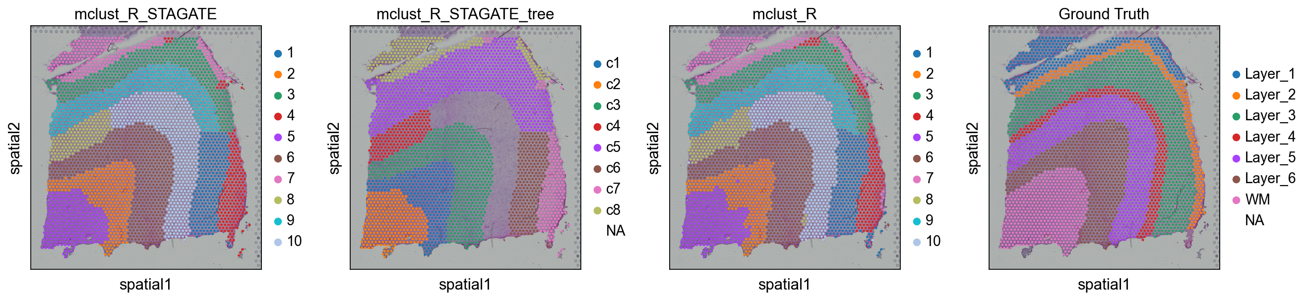
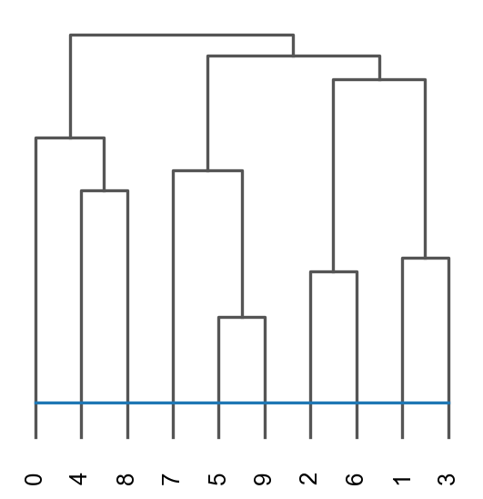
ov.utils.cluster(adata,use_rep='STAGATE',method='mclust_R',n_components=10,                 random_state=112,                )adata.obs['mclust_R_STAGATE'] = ov.utils.refine_label(adata, radius=30, key='mclust_R') adata.obs['mclust_R_STAGATE']=adata.obs['mclust_R_STAGATE'].astype('category')res=ov.space.merge_cluster(adata,groupby='mclust_R_STAGATE',use_rep='STAGATE',                  threshold=0.005,plot=True)

fitting ...
  |======================================================================| 100%
finished: found 10 clusters and added
    'mclust', the cluster labels (adata.obs, categorical)
Storing dendrogram info using `.uns['dendrogram_mclust_R_STAGATE']`
The merged cluster information is stored in adata.obs["mclust_R_STAGATE_tree"].

sc.pl.spatial(adata, color=['mclust_R_STAGATE','mclust_R_STAGATE_tree','mclust_R','Ground Truth'])

Denoising

adata.var.sort_values('PI',ascending=False).head(5)

	gene_ids	feature_types	genome	n_cells_by_counts	mean_counts	log1p_mean_counts	pct_dropout_by_counts	total_counts	log1p_total_counts	n_cells	SEP	SIG	PI	Moran_I	Geary_C	p_norm	p_rand	fdr_norm	fdr_rand	space_variable_features
MBP	ENSG00000197971	Gene Expression	GRCh38	3411	15.419075	2.798444	1.416185	53350.0	10.884648	3411	0.823299	0.214148	1.000000	0.910362	0.092733	0.0	0.0	0.0	0.0	True
GFAP	ENSG00000131095	Gene Expression	GRCh38	2938	3.930347	1.595409	15.086705	13599.0	9.517825	2938	0.694169	0.129941	0.587889	0.743831	0.255528	0.0	0.0	0.0	0.0	True
PLP1	ENSG00000123560	Gene Expression	GRCh38	3214	9.255780	2.327842	7.109827	32025.0	10.374304	3214	0.668771	0.099919	0.478698	0.737326	0.264750	0.0	0.0	0.0	0.0	True
MT-ND1	ENSG00000198888	Gene Expression	GRCh38	3460	74.200577	4.320159	0.000000	256734.0	12.455800	3460	0.362000	0.163292	0.359299	0.740392	0.262487	0.0	0.0	0.0	0.0	True
MT-CO1	ENSG00000198804	Gene Expression	GRCh38	3460	115.025436	4.753809	0.000000	397988.0	12.894179	3460	0.472005	0.100106	0.338241	0.755924	0.246897	0.0	0.0	0.0	0.0	True

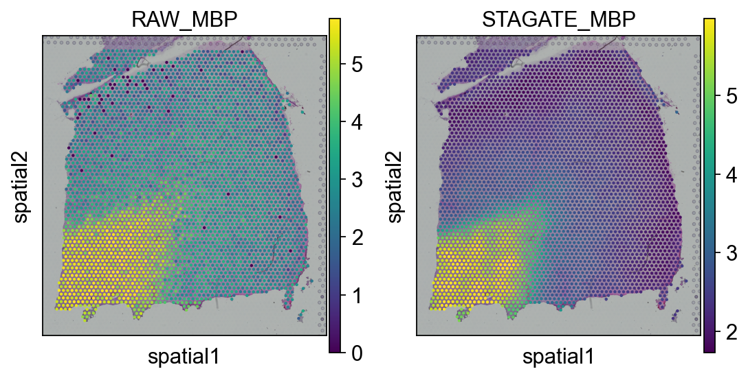
plot_gene = 'MBP'import matplotlib.pyplot as pltfig, axs = plt.subplots(1, 2, figsize=(8, 4))sc.pl.spatial(adata, img_key="hires", color=plot_gene, show=False, ax=axs[0], title='RAW_'+plot_gene, vmax='p99')sc.pl.spatial(adata, img_key="hires", color=plot_gene, show=False, ax=axs[1], title='STAGATE_'+plot_gene, layer='STAGATE_ReX', vmax='p99')

[<AxesSubplot: title={'center': 'STAGATE_MBP'}, xlabel='spatial1', ylabel='spatial2'>]

Method4: CASTCAST would be a great algorithm 如果 your spatial transcriptome is 在 单细胞 resolution 和 在 multiple slices.

methods_kwargs={}methods_kwargs['CAST']={    'output_path_t':'result/CAST_gas/output',    'device':'cuda:0',    'gpu_t':0}adata=ov.space.clusters(adata,                  methods=['CAST'],                 methods_kwargs=methods_kwargs)

The CAST method is used to embed the spatial data.
normalizing counts per cell
    finished (0:00:00)
Constructing delaunay graphs for 1 samples...
Training on cuda:0...
Finished.
The embedding, log, model files were saved to result/CAST_gas/output
The CAST embedding are stored in adata.obsm["X_cast"]. 
Shape: (3460, 512)

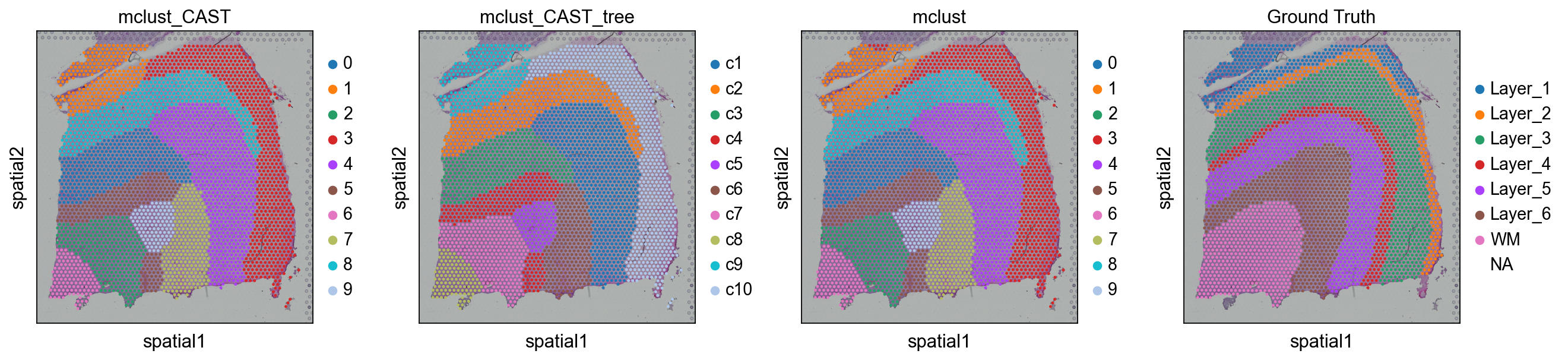
ov.utils.cluster(adata,use_rep='X_cast',method='mclust',n_components=10,                 modelNames='EEV', random_state=42,                )adata.obs['mclust_CAST'] = ov.utils.refine_label(adata, radius=50, key='mclust') adata.obs['mclust_CAST']=adata.obs['mclust_CAST'].astype('category')

running GaussianMixture clustering
finished: found 10 clusters and added
    'mclust', the cluster labels (adata.obs, categorical)

res=ov.space.merge_cluster(adata,groupby='mclust_CAST',use_rep='X_cast',                  threshold=0.1,plot=True)

Storing dendrogram info using `.uns['dendrogram_mclust_CAST']`
The merged cluster information is stored in adata.obs["mclust_CAST_tree"].

sc.pl.spatial(adata, color=['mclust_CAST','mclust_CAST_tree','mclust','Ground Truth'])

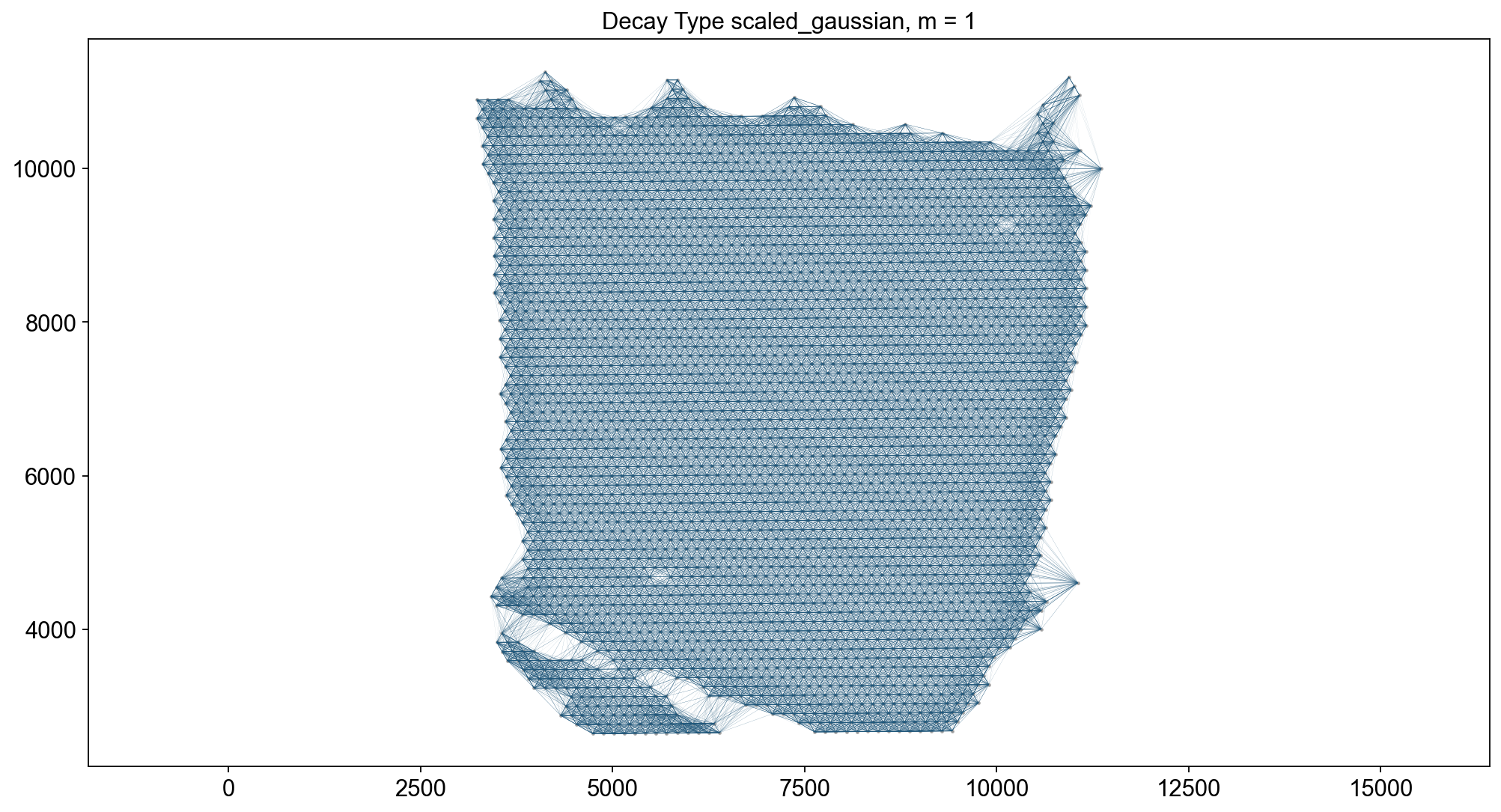
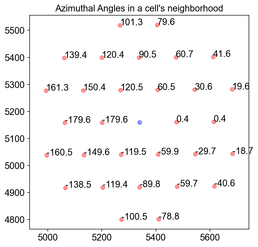
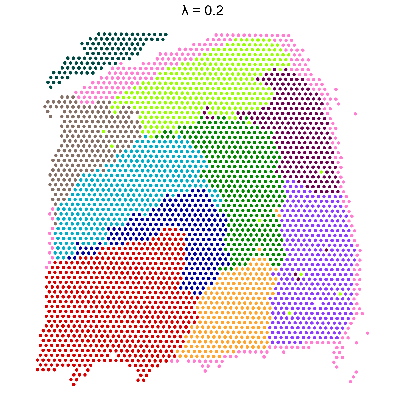
Method5: Banksy

methods_kwargs={}methods_kwargs['Banksy']={    'num_neighbours':15,    'nbr_weight_decay':'scaled_gaussian',    'max_m':1,    'lambda_list':[0.2],    'resolutions':[0.8],    'add_nonspatial':False,    'variance_balance':False,    'match_labels':False,    'filepath':'tmp/banksy',}adata=ov.space.clusters(    adata,    methods=['Banksy'],    methods_kwargs=methods_kwargs)

Median distance to closest cell = 137.00364958642524

---- Ran median_dist_to_nearest_neighbour in 0.01 s ----

---- Ran generate_spatial_distance_graph in 0.01 s ----

---- Ran row_normalize in 0.01 s ----

---- Ran generate_spatial_weights_fixed_nbrs in 0.06 s ----

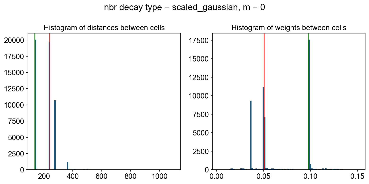
----- Plotting Edge Histograms for m = 0 -----

Edge weights (distances between cells): median = 238.76766950322232, mode = 137.00364958642524

---- Ran plot_edge_histogram in 0.04 s ----


Edge weights (weights between cells): median = 0.05057751576626019, mode = 0.09776579868038085

---- Ran plot_edge_histogram in 0.03 s ----

---- Ran generate_spatial_distance_graph in 0.02 s ----

---- Ran theta_from_spatial_graph in 0.02 s ----

---- Ran row_normalize in 0.01 s ----

---- Ran generate_spatial_weights_fixed_nbrs in 0.09 s ----

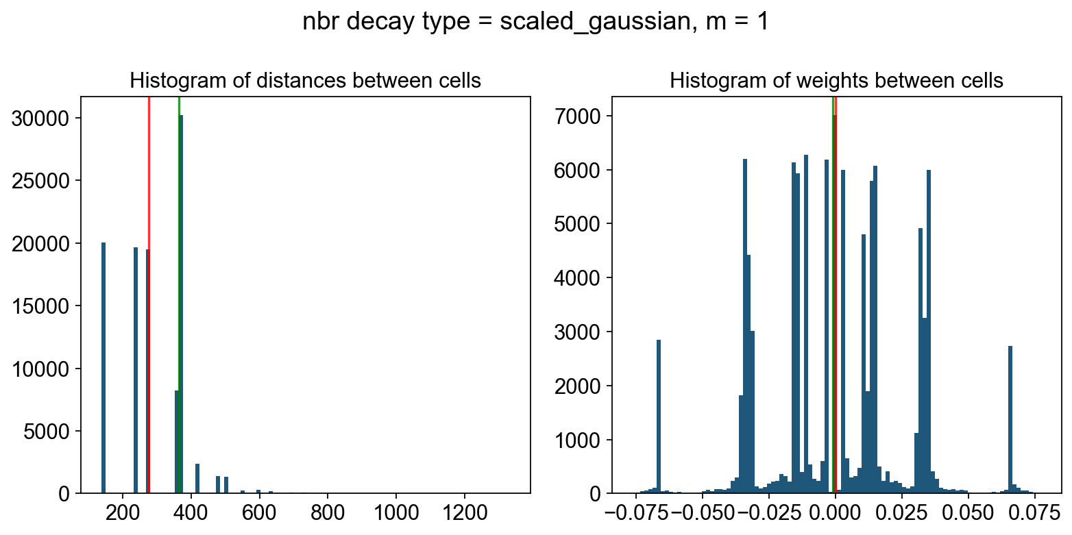
----- Plotting Edge Histograms for m = 1 -----

Edge weights (distances between cells): median = 276.2354068543712, mode = 364.36272904465324

---- Ran plot_edge_histogram in 0.04 s ----


Edge weights (weights between cells): median = (-5.2515238544983064e-05+0.008384965165521282j), mode = -0.001080415232691187

---- Ran plot_edge_histogram in 0.04 s ----

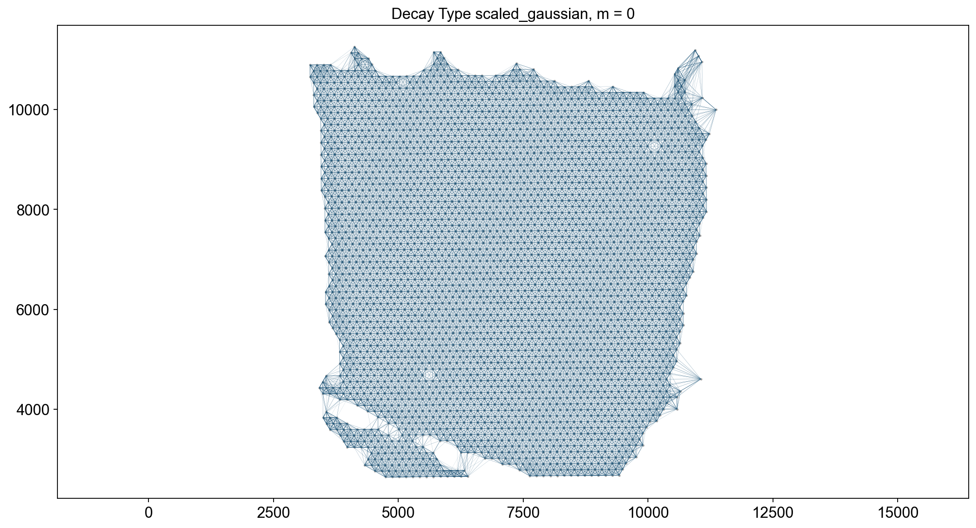
----- Plotting Weights Graph -----
Maximum weight: 0.15104274121695466

---- Ran plot_graph_weights in 0.33 s ----

Maximum weight: (0.07735695704637852+0.0005605576383513445j)

---- Ran plot_graph_weights in 0.64 s ----

----- Plotting theta Graph -----
Runtime Jan-08-2026-00-33

10747 genes to be analysed:
Gene List:
Index(['NOC2L', 'KLHL17', 'HES4', 'ISG15', 'AGRN', 'C1orf159', 'SDF4',
       'B3GALT6', 'UBE2J2', 'SCNN1D',
       ...
       'MT-ATP8', 'MT-ATP6', 'MT-CO3', 'MT-ND3', 'MT-ND4L', 'MT-ND4', 'MT-ND5',
       'MT-ND6', 'MT-CYB', 'AC007325.4'],
      dtype='object', length=10747)

Check if X contains only finite (non-NAN) values
Decay Type: scaled_gaussian
Weights Object: {'weights': {0: <3460x3460 sparse matrix of type '<class 'numpy.float64'>'
	with 51900 stored elements in Compressed Sparse Row format>, 1: <3460x3460 sparse matrix of type '<class 'numpy.complex128'>'
	with 103800 stored elements in Compressed Sparse Row format>}}

Nbr matrix | Mean: 0.27 | Std: 0.42
Size of Nbr | Shape: (3460, 10747)
Top 3 entries of Nbr Mat:

[[0.34965952 0.10314547 0.25060342]
 [0.03750811 0.         0.3298474 ]
 [0.24471095 0.20862651 0.39286428]]

AGF matrix | Mean: 0.09 | Std: 0.09
Size of AGF mat (m = 1) | Shape: (3460, 10747)
Top entries of AGF:
[[0.09590092 0.07119773 0.09831454]
 [0.02268589 0.0157818  0.08236299]
 [0.10259601 0.14517428 0.09064761]]
Ran 'Create BANKSY Matrix' in 0.1 mins

Cell by gene matrix has shape (3460, 10747)

Scale factors squared: [0.8        0.13333333 0.06666667]
Scale factors: [0.89442719 0.36514837 0.25819889]
Shape of BANKSY matrix: (3460, 32241)
Type of banksy_matrix: <class 'anndata._core.anndata.AnnData'>

Current decay types: ['scaled_gaussian']

Reducing dims of dataset in (Index = scaled_gaussian, lambda = 0.2)
==================================================

Setting the total number of PC = 20
Original shape of matrix: (3460, 32241)
Reduced shape of matrix: (3460, 20)
------------------------------------------------------------
min_value = -32.08530858175148, mean = 4.189327112574001e-17, max = 71.19746300495925

Conducting clustering with Leiden Parition
Decay type: scaled_gaussian
Neighbourhood Contribution (Lambda Parameter): 0.2
reduced_pc_20 

PCA dims to analyse: [20]

====================================================================================================
Setting up partitioner for (nbr decay = scaled_gaussian), Neighbourhood contribution = 0.2, PCA dimensions = 20)
====================================================================================================


Nearest-neighbour weighted graph (dtype: float64, shape: (3460, 3460)) has 173000 nonzero entries.
---- Ran find_nn in 0.15 s ----


Nearest-neighbour connectivity graph (dtype: int16, shape: (3460, 3460)) has 173000 nonzero entries.

(after computing shared NN)
Allowing nearest neighbours only reduced the number of shared NN from 1068214 to 172908.


Shared nearest-neighbour (connections only) graph (dtype: int16, shape: (3460, 3460)) has 171525 nonzero entries.

Shared nearest-neighbour (number of shared neighbours as weights) graph (dtype: int16, shape: (3460, 3460)) has 171525 nonzero entries.

sNN graph data:
[28 10 17 ... 14 24 12]

---- Ran shared_nn in 0.08 s ----


-- Multiplying sNN connectivity by weights --


shared NN with distance-based weights graph (dtype: float64, shape: (3460, 3460)) has 171525 nonzero entries.
shared NN weighted graph data: [0.10762001 0.10781988 0.10841317 ... 0.11061305 0.1362395  0.13745543]

Converting graph (dtype: float64, shape: (3460, 3460)) has 171525 nonzero entries.
---- Ran csr_to_igraph in 0.03 s ----


Resolution: 0.8
------------------------------

---- Partitioned BANKSY graph ----
modularity: 0.77
11 unique labels:
[ 0  1  2  3  4  5  6  7  8  9 10]

---- Ran partition in 0.82 s ----

No annotated labels

After sorting Dataframe
Shape of dataframe: (1, 7)
Anndata AxisArrays with keys: reduced_pc_20

	decay	lambda_param	num_pcs	resolution	num_labels	labels	adata
scaled_gaussian_pc20_nc0.20_r0.80	scaled_gaussian	0.2	20	0.8	11	Label object:\nNumber of labels: 11, number of...	[[[View of AnnData object with n_obs × n_vars ...

adata.obsm['X_banksy']=adata.obsm['X_banksy_scaled_gaussian_pc20_nc0.20_r0.80']

ov.utils.cluster(adata,use_rep='X_banksy',method='mclust',n_components=10,                 modelNames='EEV', random_state=42,                )adata.obs['mclust_banksy'] = ov.utils.refine_label(adata, radius=50, key='mclust') adata.obs['mclust_banksy']=adata.obs['mclust_banksy'].astype('category')

running GaussianMixture clustering
finished: found 10 clusters and added
    'mclust', the cluster labels (adata.obs, categorical)

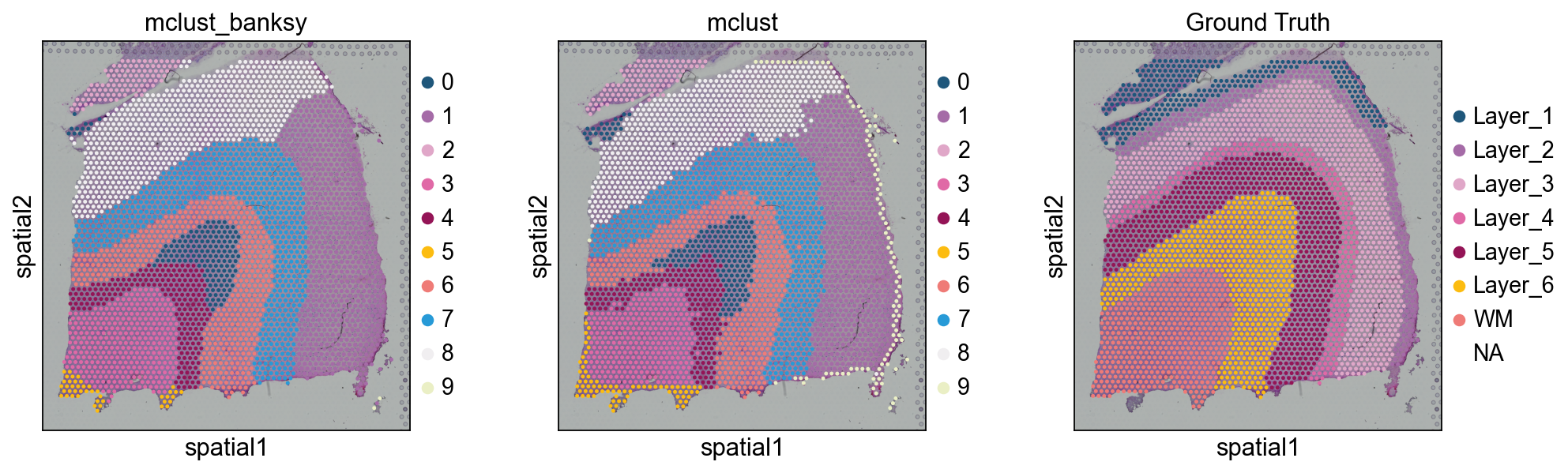
sc.pl.spatial(adata,               color=['mclust_banksy','mclust','Ground Truth']             )

评估 clusterWe use ARI 到 评估 该 scoring 的 our clusters against 该 true valuesWhile it appears 那 STAGATE works best, note 那 此 is only 在 此 数据集.- 如果 your 数据 is 点位-level resolution, GraphST, BINARY 和 STAGATE would be 好的 algorithms 到 use- BINARY 和 CAST would be 好的 algorithms 如果 your 数据 is NanoString 或 other 单细胞 resolution

from sklearn.metrics.cluster import adjusted_rand_scoreobs_df = adata.obs.dropna()# GraphSTARI = adjusted_rand_score(obs_df['mclust_GraphST'], obs_df['Ground Truth'])print('mclust_GraphST: Adjusted rand index = %.2f' %ARI)ARI = adjusted_rand_score(obs_df['mclust_R_GraphST'], obs_df['Ground Truth'])print('mclust_R_GraphST: Adjusted rand index = %.2f' %ARI)ARI = adjusted_rand_score(obs_df['mclust_R_STAGATE'], obs_df['Ground Truth'])print('mclust_STAGATE: Adjusted rand index = %.2f' %ARI)ARI = adjusted_rand_score(obs_df['mclust_BINARY'], obs_df['Ground Truth'])print('mclust_BINARY: Adjusted rand index = %.2f' %ARI)ARI = adjusted_rand_score(obs_df['mclustpy_BINARY'], obs_df['Ground Truth'])print('mclustpy_BINARY: Adjusted rand index = %.2f' %ARI)ARI = adjusted_rand_score(obs_df['mclust_CAST'], obs_df['Ground Truth'])print('mclust_CAST: Adjusted rand index = %.2f' %ARI)

mclust_GraphST: Adjusted rand index = 0.37
mclust_R_GraphST: Adjusted rand index = 0.42
mclust_STAGATE: Adjusted rand index = 0.53
mclust_BINARY: Adjusted rand index = 0.47
mclustpy_BINARY: Adjusted rand index = 0.43
mclust_CAST: Adjusted rand index = 0.40

from sklearn.metrics.cluster import adjusted_rand_scoreobs_df = adata.obs.dropna()ARI = adjusted_rand_score(obs_df['mclust_banksy'], obs_df['Ground Truth'])print('mclust_banksy: Adjusted rand index = %.2f' %ARI)

mclust_banksy: Adjusted rand index = 0.46