
单细胞RNA-seq懒惰分析#
我们都知道单细胞分析的预处理是繁琐和乏味的。在OmicVerse的未来开发中,我们将逐步引入代理来使整个分析完全自动化。在版本1.7.0中,我们已经支持完全自动化的数据预处理,在下一个版本中我们期望自动化细胞注释。
我们提供了一个函数
omicverse.single.lazy,可以自动预处理单细胞数据,参数可调。我们提供了一个分析报告生成器
omicverse.single.generate_scRNA_report,类似于MultiQC,用于可视化我们的预处理结果。此外,对于OmicVerse中调用的每一个分析,你现在可以通过
ov.generate_reference_table生成参考文献引用和DOI。
import scanpy as sc
#import pertpy as pt
import omicverse as ov
ov.plot_set()
🔬 Starting plot initialization...
🧬 Detecting CUDA devices…
✅ [GPU 0] NVIDIA H100 80GB HBM3
    • Total memory: 79.1 GB
    • Compute capability: 9.0

   ____            _     _    __
  / __ \____ ___  (_)___| |  / /__  _____________
 / / / / __ `__ \/ / ___/ | / / _ \/ ___/ ___/ _ \
/ /_/ / / / / / / / /__ | |/ /  __/ /  (__  )  __/
\____/_/ /_/ /_/_/\___/ |___/\___/_/  /____/\___/

🔖 Version: 1.7.0   📚 Tutorials: https://omicverse.readthedocs.io/
✅ plot_set complete.
数据准备#
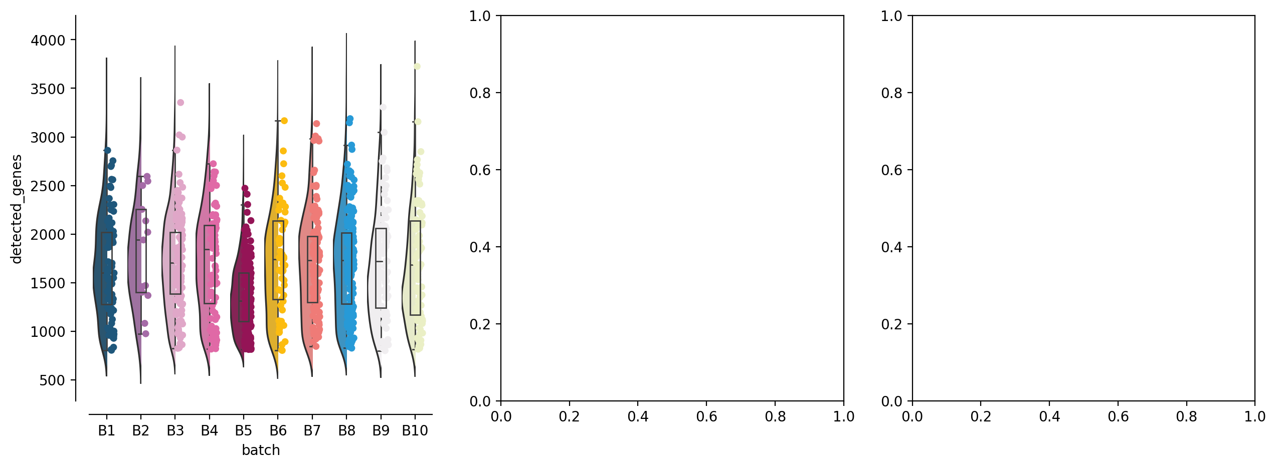
我们在下面的示例中使用的数据来自Haber等人,2017年。它包含来自不同条件下小鼠小肠上皮的样本。我们首先加载原始细胞级别的数据。该数据集包含9842个细胞的基因表达。它们用样本标识符(batch)、受试者的条件和每个细胞的类型(cell_label)进行注释。
import pertpy as pt
adata = pt.dt.haber_2017_regions()
adata
ov.settings.cpu_gpu_mixed_init()
CPU-GPU mixed mode activated
懒惰分析#
目前仅支持人类和小鼠物种;我们可能在未来添加更多物种。如果不指定任何参数,分析将使用默认设置运行。
%time
adata=ov.single.lazy(adata,species='mouse',sample_key='batch')
CPU times: user 2 μs, sys: 0 ns, total: 2 μs
Wall time: 4.53 μs
🔧 The mode of lazy is cpu-gpu-mixed
✅ All packages used in lazy are installed
❌ QC step didn't start, we will start it now
🔧 The argument of qc we set
   mito_perc: 0.2
   nUMIs: 500
   detected_genes: 250
   doublets_method: scrublet
   batch_key: batch

⚙️ Using torch CPU/GPU mixed mode...
📊 [GPU 0] ------------------------------ 4/81559 MiB (0.0%)
Calculate QC metrics
End calculation of QC metrics.
Original cell number: 9842
!!!It should be noted that the `scrublet` detection is too old and             may not work properly.!!!
!!!if you want to use novel doublet detection,             please set `doublets_method=sccomposite`!!!
Begin of post doublets removal and QC plot using`scrublet`
Running Scrublet🔍
filtered out 3076 genes that are detected in less than 3 cells
normalizing counts per cell
    finished (0:00:00)
extracting highly variable genes
    finished (0:00:00)
--> added
    'highly_variable', boolean vector (adata.var)
    'means', float vector (adata.var)
    'dispersions', float vector (adata.var)
    'dispersions_norm', float vector (adata.var)
normalizing counts per cell
    finished (0:00:00)
normalizing counts per cell
    finished (0:00:00)
Embedding transcriptomes using PCA...
    using data matrix X directly
Automatically set threshold at doublet score = 0.24
Detected doublet rate = 0.6%
Estimated detectable doublet fraction = 5.1%
Overall doublet rate:
	Expected   = 5.0%
	Estimated  = 11.8%
filtered out 3227 genes that are detected in less than 3 cells
normalizing counts per cell
    finished (0:00:00)
extracting highly variable genes
    finished (0:00:00)
--> added
    'highly_variable', boolean vector (adata.var)
    'means', float vector (adata.var)
    'dispersions', float vector (adata.var)
    'dispersions_norm', float vector (adata.var)
normalizing counts per cell
    finished (0:00:00)
normalizing counts per cell
    finished (0:00:00)
Embedding transcriptomes using PCA...
    using data matrix X directly
Automatically set threshold at doublet score = 0.24
Detected doublet rate = 0.3%
Estimated detectable doublet fraction = 30.8%
Overall doublet rate:
	Expected   = 5.0%
	Estimated  = 1.0%
filtered out 4938 genes that are detected in less than 3 cells
normalizing counts per cell
    finished (0:00:00)
extracting highly variable genes
    finished (0:00:00)
--> added
    'highly_variable', boolean vector (adata.var)
    'means', float vector (adata.var)
    'dispersions', float vector (adata.var)
    'dispersions_norm', float vector (adata.var)
normalizing counts per cell
    finished (0:00:00)
normalizing counts per cell
    finished (0:00:00)
Embedding transcriptomes using PCA...
    using data matrix X directly
Automatically set threshold at doublet score = 0.13
Detected doublet rate = 2.5%
Estimated detectable doublet fraction = 28.0%
Overall doublet rate:
	Expected   = 5.0%
	Estimated  = 8.9%
filtered out 2755 genes that are detected in less than 3 cells
normalizing counts per cell
    finished (0:00:00)
extracting highly variable genes
    finished (0:00:00)
--> added
    'highly_variable', boolean vector (adata.var)
    'means', float vector (adata.var)
    'dispersions', float vector (adata.var)
    'dispersions_norm', float vector (adata.var)
normalizing counts per cell
    finished (0:00:00)
normalizing counts per cell
    finished (0:00:00)
Embedding transcriptomes using PCA...
    using data matrix X directly
Automatically set threshold at doublet score = 0.29
Detected doublet rate = 0.2%
Estimated detectable doublet fraction = 3.9%
Overall doublet rate:
	Expected   = 5.0%
	Estimated  = 4.1%
filtered out 3179 genes that are detected in less than 3 cells
normalizing counts per cell
    finished (0:00:00)
extracting highly variable genes
    finished (0:00:00)
--> added
    'highly_variable', boolean vector (adata.var)
    'means', float vector (adata.var)
    'dispersions', float vector (adata.var)
    'dispersions_norm', float vector (adata.var)
normalizing counts per cell
    finished (0:00:00)
normalizing counts per cell
    finished (0:00:00)
Embedding transcriptomes using PCA...
    using data matrix X directly
Automatically set threshold at doublet score = 0.25
Detected doublet rate = 0.6%
Estimated detectable doublet fraction = 21.1%
Overall doublet rate:
	Expected   = 5.0%
	Estimated  = 3.0%
filtered out 2892 genes that are detected in less than 3 cells
normalizing counts per cell
    finished (0:00:00)
extracting highly variable genes
    finished (0:00:00)
--> added
    'highly_variable', boolean vector (adata.var)
    'means', float vector (adata.var)
    'dispersions', float vector (adata.var)
    'dispersions_norm', float vector (adata.var)
normalizing counts per cell
    finished (0:00:00)
normalizing counts per cell
    finished (0:00:00)
Embedding transcriptomes using PCA...
    using data matrix X directly
Automatically set threshold at doublet score = 0.30
Detected doublet rate = 0.3%
Estimated detectable doublet fraction = 2.2%
Overall doublet rate:
	Expected   = 5.0%
	Estimated  = 11.9%
filtered out 3305 genes that are detected in less than 3 cells
normalizing counts per cell
    finished (0:00:00)
extracting highly variable genes
    finished (0:00:00)
--> added
    'highly_variable', boolean vector (adata.var)
    'means', float vector (adata.var)
    'dispersions', float vector (adata.var)
    'dispersions_norm', float vector (adata.var)
normalizing counts per cell
    finished (0:00:00)
normalizing counts per cell
    finished (0:00:00)
Embedding transcriptomes using PCA...
    using data matrix X directly
Automatically set threshold at doublet score = 0.23
Detected doublet rate = 0.6%
Estimated detectable doublet fraction = 12.9%
Overall doublet rate:
	Expected   = 5.0%
	Estimated  = 4.9%
filtered out 2804 genes that are detected in less than 3 cells
normalizing counts per cell
    finished (0:00:00)
extracting highly variable genes
    finished (0:00:00)
--> added
    'highly_variable', boolean vector (adata.var)
    'means', float vector (adata.var)
    'dispersions', float vector (adata.var)
    'dispersions_norm', float vector (adata.var)
normalizing counts per cell
    finished (0:00:00)
normalizing counts per cell
    finished (0:00:00)
Embedding transcriptomes using PCA...
    using data matrix X directly
Automatically set threshold at doublet score = 0.27
Detected doublet rate = 0.6%
Estimated detectable doublet fraction = 17.6%
Overall doublet rate:
	Expected   = 5.0%
	Estimated  = 3.4%
filtered out 2682 genes that are detected in less than 3 cells
normalizing counts per cell
    finished (0:00:00)
extracting highly variable genes
    finished (0:00:00)
--> added
    'highly_variable', boolean vector (adata.var)
    'means', float vector (adata.var)
    'dispersions', float vector (adata.var)
    'dispersions_norm', float vector (adata.var)
normalizing counts per cell
    finished (0:00:00)
normalizing counts per cell
    finished (0:00:00)
Embedding transcriptomes using PCA...
    using data matrix X directly
Automatically set threshold at doublet score = 0.31
Detected doublet rate = 0.5%
Estimated detectable doublet fraction = 6.2%
Overall doublet rate:
	Expected   = 5.0%
	Estimated  = 8.4%
filtered out 3331 genes that are detected in less than 3 cells
normalizing counts per cell
    finished (0:00:00)
extracting highly variable genes
    finished (0:00:00)
--> added
    'highly_variable', boolean vector (adata.var)
    'means', float vector (adata.var)
    'dispersions', float vector (adata.var)
    'dispersions_norm', float vector (adata.var)
normalizing counts per cell
    finished (0:00:00)
normalizing counts per cell
    finished (0:00:00)
Embedding transcriptomes using PCA...
    using data matrix X directly
Automatically set threshold at doublet score = 0.23
Detected doublet rate = 0.0%
Estimated detectable doublet fraction = 28.9%
Overall doublet rate:
	Expected   = 5.0%
	Estimated  = 0.0%
    Scrublet finished✅ (0:00:26)
Cells retained after scrublet: 9798, 44 removed.
End of post doublets removal and QC plots.
Filters application (seurat or mads)
Lower treshold, nUMIs: 500; filtered-out-cells:         0
Lower treshold, n genes: 250; filtered-out-cells:         0
Lower treshold, mito %: 0.2; filtered-out-cells:         0
Filters applicated.
Total cell filtered out with this last --mode seurat QC (and its     chosen options): 0
Cells retained after scrublet and seurat filtering: 9798, 44 removed.
filtered out 626 genes that are detected in less than 3 cells
❌ Preprocess step didn't start, we will start it now
🔧 The argument of preprocess we set
   mode: shiftlog|pearson
   n_HVGs: 2000
   target_sum: 500000.0

Begin robust gene identification
After filtration, 14589/14589 genes are kept.     Among 14589 genes, 14589 genes are robust.
End of robust gene identification.
Begin size normalization: shiftlog and HVGs selection pearson
normalizing counts per cell. The following highly-expressed genes are not considered during normalization factor computation:
['Cck', 'Defa24', 'Fabp6', 'Gcg', 'Ghrl', 'Gip', 'Nts', 'Reg3b', 'Reg3g', 'Reg4', 'Sct', 'Spink4', 'Sst', 'Tff3', 'Zg16']
    finished (0:00:00)
extracting highly variable genes
--> added
    'highly_variable', boolean vector (adata.var)
    'highly_variable_rank', float vector (adata.var)
    'highly_variable_nbatches', int vector (adata.var)
    'highly_variable_intersection', boolean vector (adata.var)
    'means', float vector (adata.var)
    'variances', float vector (adata.var)
    'residual_variances', float vector (adata.var)
Time to analyze data in cpu: 9.195535898208618 seconds.
End of size normalization: shiftlog and HVGs selection pearson
❌ Scaled step didn't start, we will start it now
❌ PCA step didn't start, we will start it now
🔧 The argument of PCA we set
   layer: scaled
   n_pcs: 50
   use_highly_variable: True

🚀 Using GPU to calculate PCA...
📊 [GPU 0] ------------------------------ 4/81559 MiB (0.0%)
computing PCA🔍
    with n_comps=50
[KeOps] Compiling cuda jit compiler engine ... OK
[pyKeOps] Compiling nvrtc binder for python ... OK
    finished✅ (0:00:17)
❌ Cell cycle scoring step didn't start, we will start it now
calculating cell cycle phase
computing score 'S_score'
    finished: added
    'S_score', score of gene set (adata.obs).
    642 total control genes are used. (0:00:00)
computing score 'G2M_score'
WARNING: genes are not in var_names and ignored: Index(['Cks2', 'Jpt1', 'Pimreg'], dtype='object')
    finished: added
    'G2M_score', score of gene set (adata.obs).
    597 total control genes are used. (0:00:00)
-->     'phase', cell cycle phase (adata.obs)
❌ Batch Correction: `Harmony` step didn't start, we will start it now
...Begin using harmony to correct batch effect
🖥️ Using Scanpy CPU to calculate neighbors...
computing neighbors
    finished: added to `.uns['neighbors']`
    `.obsp['distances']`, distances for each pair of neighbors
    `.obsp['connectivities']`, weighted adjacency matrix (0:00:25)
🔍 [2025-05-27 02:51:13] Running UMAP in 'cpu-gpu-mixed' mode...
🚀 Using torch GPU to calculate UMAP...
📊 [GPU 0] ------------------------------ 4/81559 MiB (0.0%)
computing UMAP🚀
    finished ✅: added
    'X_umap', UMAP coordinates (adata.obsm)
    'umap', UMAP parameters (adata.uns) (0:00:09)
✅ UMAP completed successfully.
⚙️ Using torch CPU/GPU mixed mode to calculate t-SNE...
📊 [GPU 0] ------------------------------ 1084/81559 MiB (1.3%)
computing tSNE🔍
    using sklearn.manifold.TSNE
    finished ✅: added
    'X_tsne', tSNE coordinates (adata.obsm)
    'tsne', tSNE parameters (adata.uns) (0:00:15)
❌ Batch Correction: `scVI` step didn't start, we will start it now
...Begin using scVI to correct batch effect
🖥️ Using Scanpy CPU to calculate neighbors...
computing neighbors
    finished: added to `.uns['neighbors']`
    `.obsp['distances']`, distances for each pair of neighbors
    `.obsp['connectivities']`, weighted adjacency matrix (0:00:02)
🔍 [2025-05-27 02:54:44] Running UMAP in 'cpu-gpu-mixed' mode...
🚀 Using torch GPU to calculate UMAP...
📊 [GPU 0] ------------------------------ 1158/81559 MiB (1.4%)
computing UMAP🚀
    finished ✅: added
    'X_umap', UMAP coordinates (adata.obsm)
    'umap', UMAP parameters (adata.uns) (0:00:03)
✅ UMAP completed successfully.
⚙️ Using torch CPU/GPU mixed mode to calculate t-SNE...
📊 [GPU 0] ------------------------------ 1234/81559 MiB (1.5%)
computing tSNE🔍
    using sklearn.manifold.TSNE
    finished ✅: added
    'X_tsne', tSNE coordinates (adata.obsm)
    'tsne', tSNE parameters (adata.uns) (0:00:24)
❌ Best Bench Correction Eval step didn't start, we will start it now
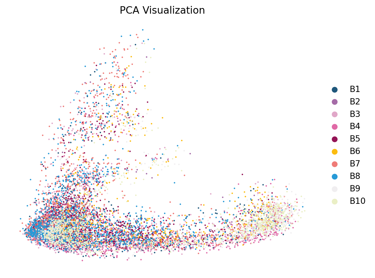
The Best Bench Correction Method is X_scVI
We can found it in `adata.uns['bench_best_res']`
❌ Best Clusters step didn't start, we will start it now
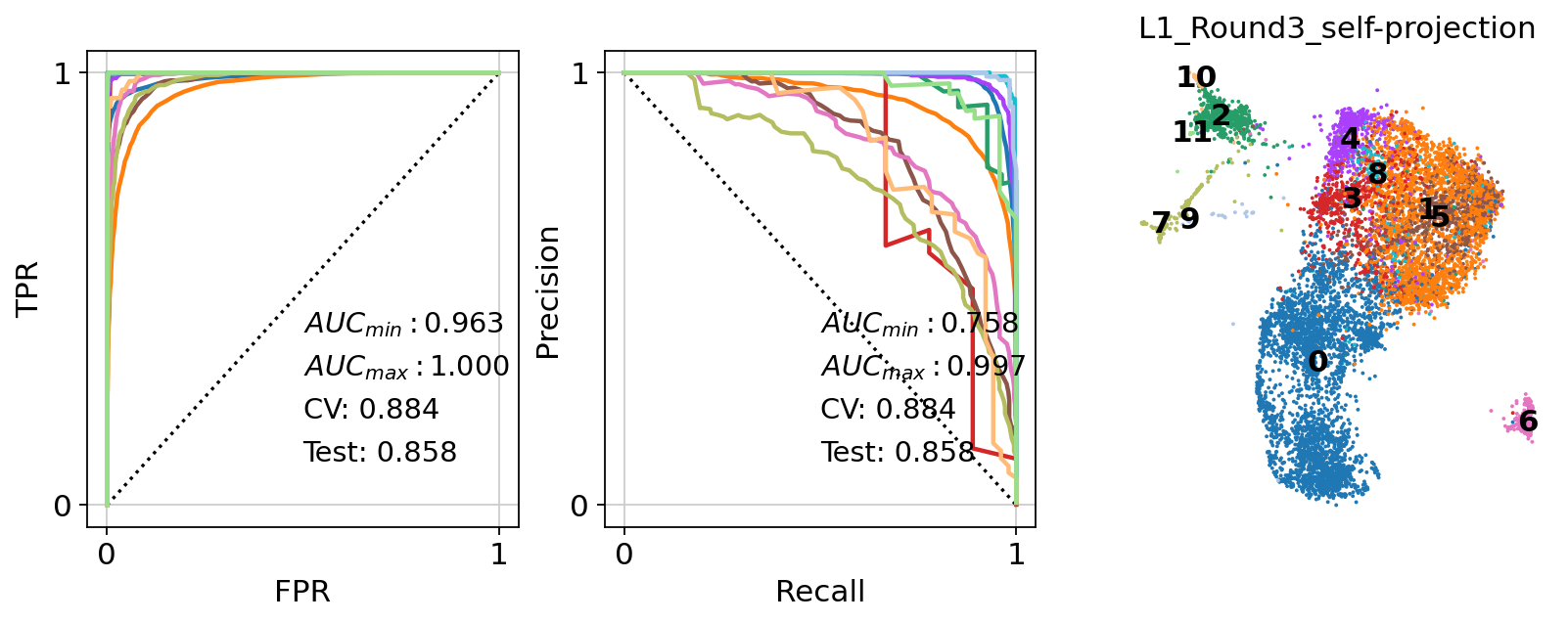
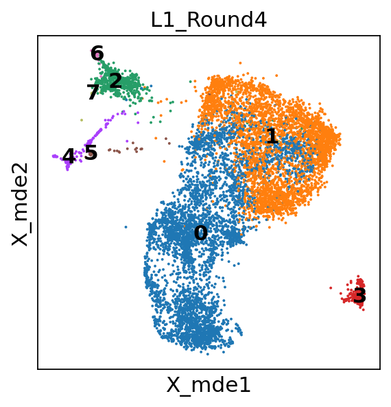
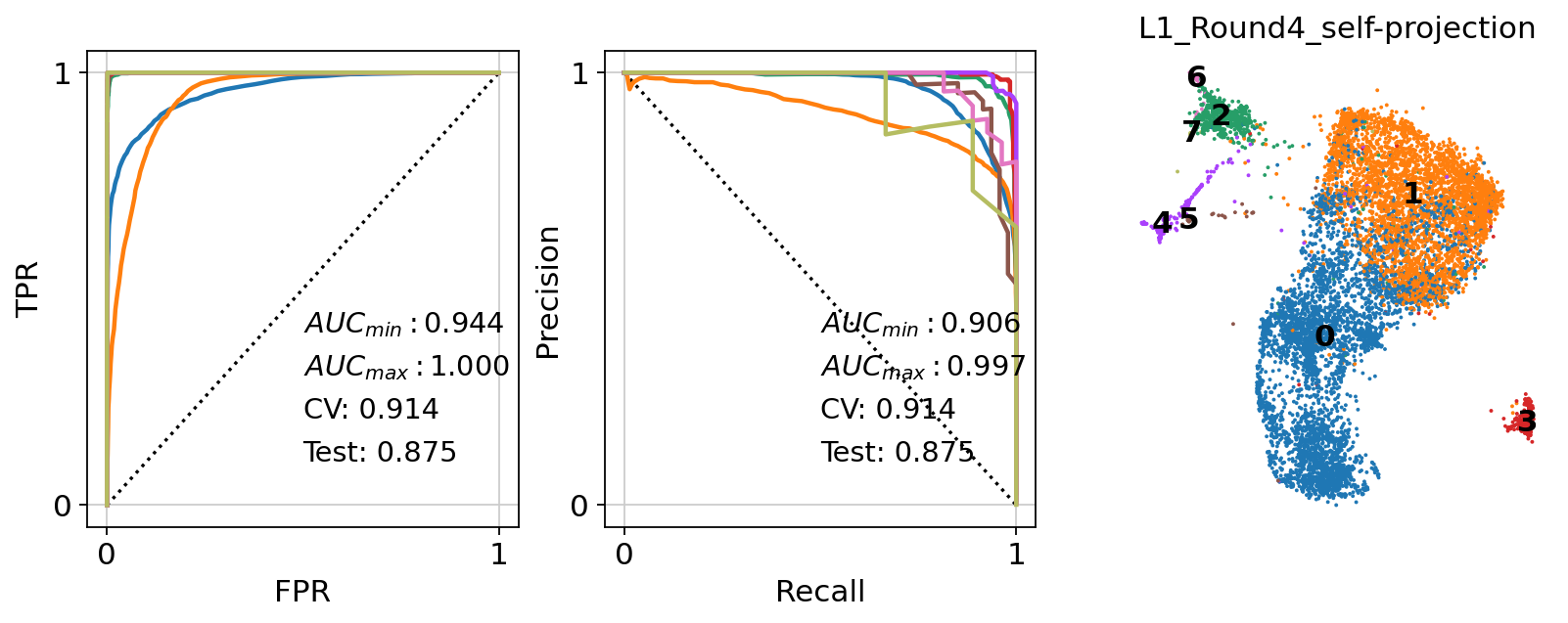
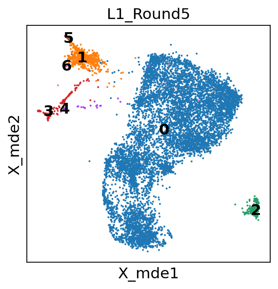
Automatic clustering using sccaf
Dimensionality using :X_scVI
computing neighbors
    finished: added to `.uns['neighbors']`
    `.obsm['X_mde']`, MDE coordinates
    `.obsp['neighbors_distances']`, distances for each pair of neighbors
    `.obsp['neighbors_connectivities']`, weighted adjacency matrix (0:00:02)
🖥️ Using Scanpy CPU to calculate neighbors...
computing neighbors
    finished: added to `.uns['neighbors']`
    `.obsp['distances']`, distances for each pair of neighbors
    `.obsp['connectivities']`, weighted adjacency matrix (0:00:02)
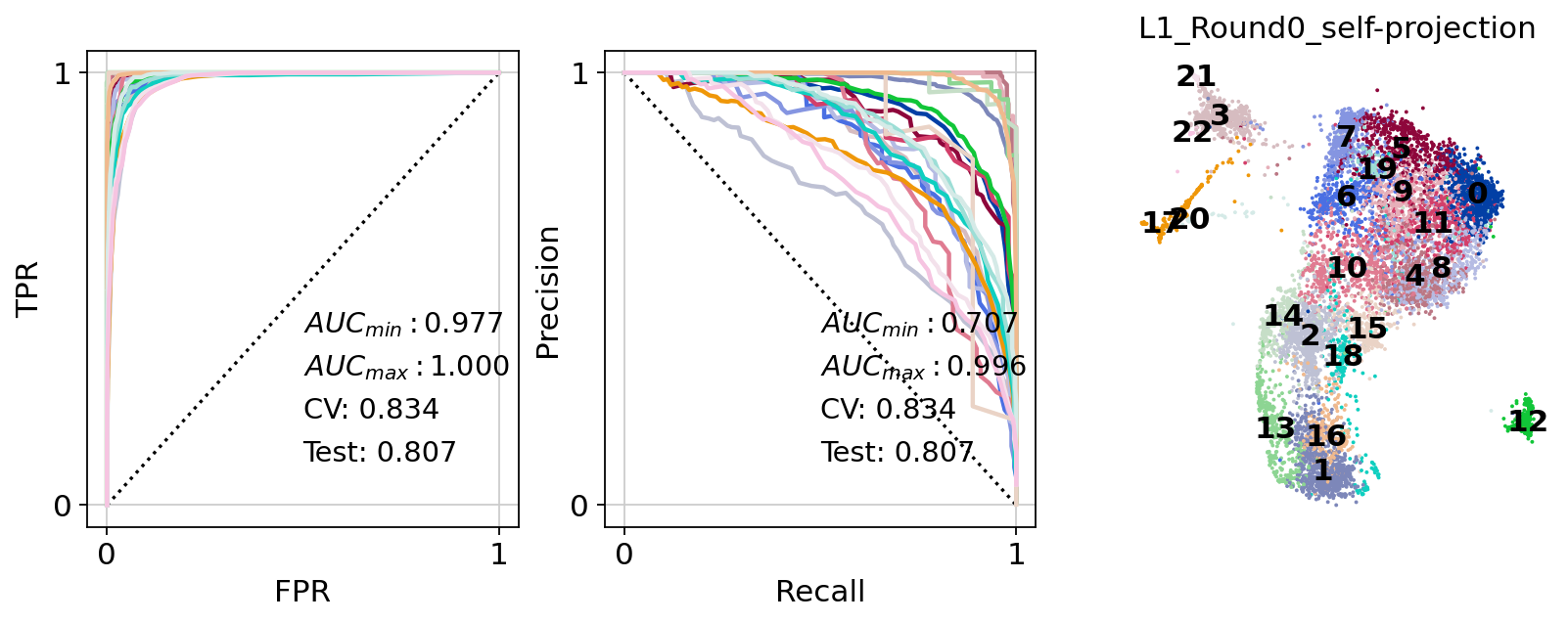
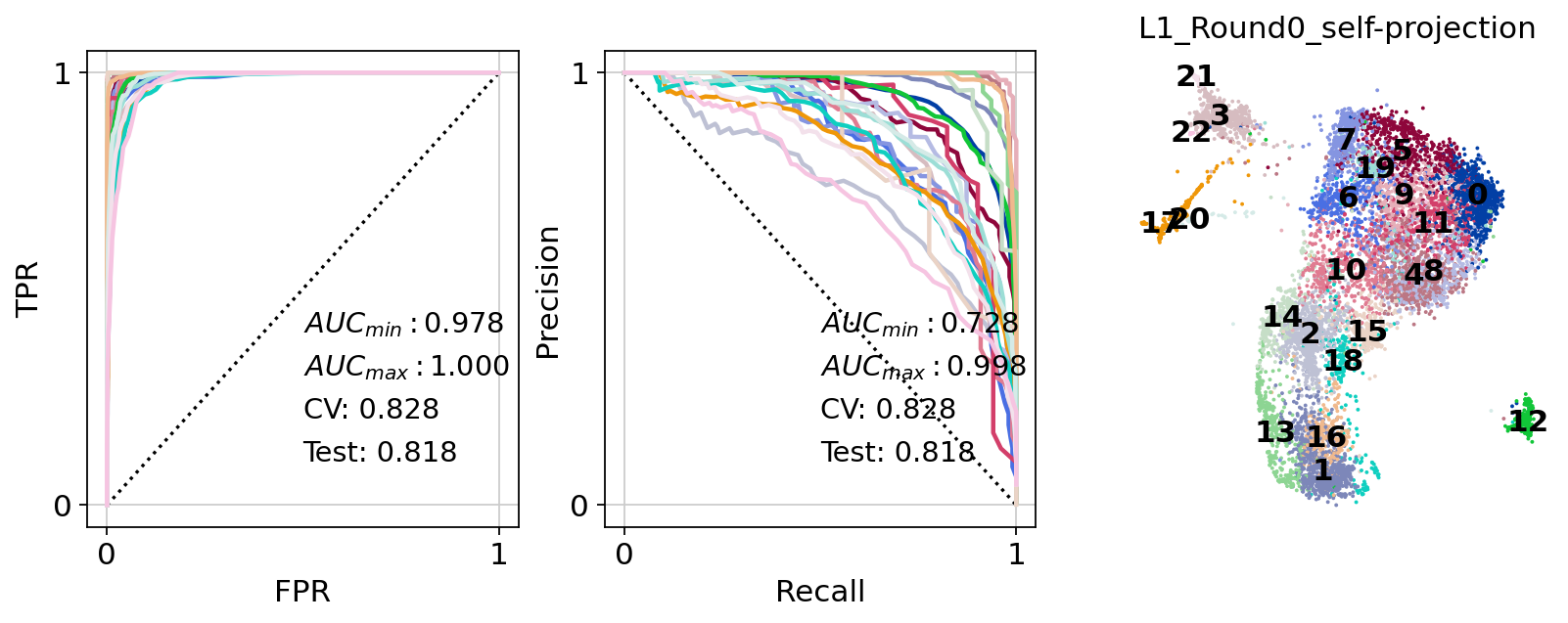
Automatic clustering using leiden for preprocessed
running Leiden clustering
    finished: found 23 clusters and added
    'leiden_r1.5', the cluster labels (adata.obs, categorical) (0:00:03)
Automatic clustering using sccaf, Times: 0
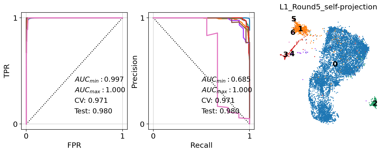
Mean CV accuracy: 0.8337
Accuracy on the training set: 1.0000
Accuracy on the hold-out set: 0.8068
Accuracy on the training set: 1.0000
Accuracy on the hold-out set: 0.8142
Accuracy on the training set: 1.0000
Accuracy on the hold-out set: 0.8030
Converge SCCAF_optimize no. cluster!
Mean CV accuracy: 0.8278
Accuracy on the training set: 1.0000
Accuracy on the hold-out set: 0.8180
Accuracy on the training set: 1.0000
Accuracy on the hold-out set: 0.7950
Accuracy on the training set: 1.0000
Accuracy on the hold-out set: 0.8111
Mean CV accuracy: 0.8311
Accuracy on the training set: 1.0000
Accuracy on the hold-out set: 0.8231
Accuracy on the training set: 1.0000
Accuracy on the hold-out set: 0.8131
Accuracy on the training set: 1.0000
Accuracy on the hold-out set: 0.8279
Converge SCCAF_optimize no. cluster!
Mean CV accuracy: 0.8231
Accuracy on the training set: 1.0000
Accuracy on the hold-out set: 0.8234
Accuracy on the training set: 1.0000
Accuracy on the hold-out set: 0.8235
Accuracy on the training set: 1.0000
Accuracy on the hold-out set: 0.8199
Mean CV accuracy: 0.8442
Accuracy on the training set: 1.0000
Accuracy on the hold-out set: 0.8340
Accuracy on the training set: 1.0000
Accuracy on the hold-out set: 0.8334
Accuracy on the training set: 1.0000
Accuracy on the hold-out set: 0.8330
Mean CV accuracy: 0.8845
Accuracy on the training set: 1.0000
Accuracy on the hold-out set: 0.8582
Accuracy on the training set: 1.0000
Accuracy on the hold-out set: 0.8548
Accuracy on the training set: 1.0000
Accuracy on the hold-out set: 0.8625
Mean CV accuracy: 0.9144
Accuracy on the training set: 1.0000
Accuracy on the hold-out set: 0.8748
Accuracy on the training set: 1.0000
Accuracy on the hold-out set: 0.8778
Accuracy on the training set: 1.0000
Accuracy on the hold-out set: 0.8907
Mean CV accuracy: 0.9710
Accuracy on the training set: 1.0000
Accuracy on the hold-out set: 0.9797
Accuracy on the training set: 1.0000
Accuracy on the hold-out set: 0.9875
Accuracy on the training set: 1.0000
Accuracy on the hold-out set: 0.9726
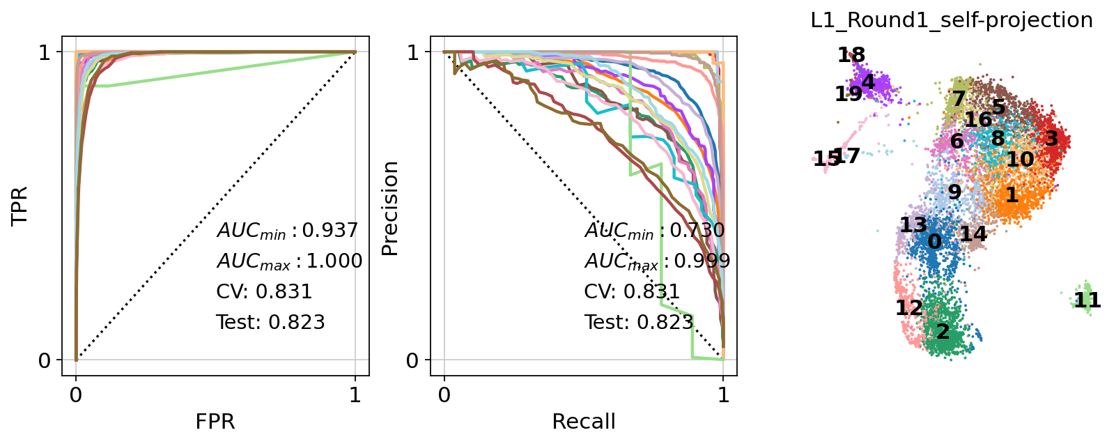
Reached the minimum accuracy!
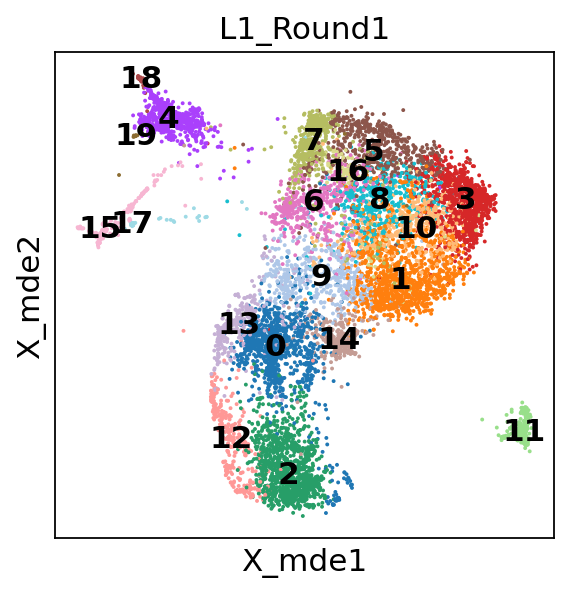
Smoothing the effect of clustering, Times: 0
running Leiden clustering
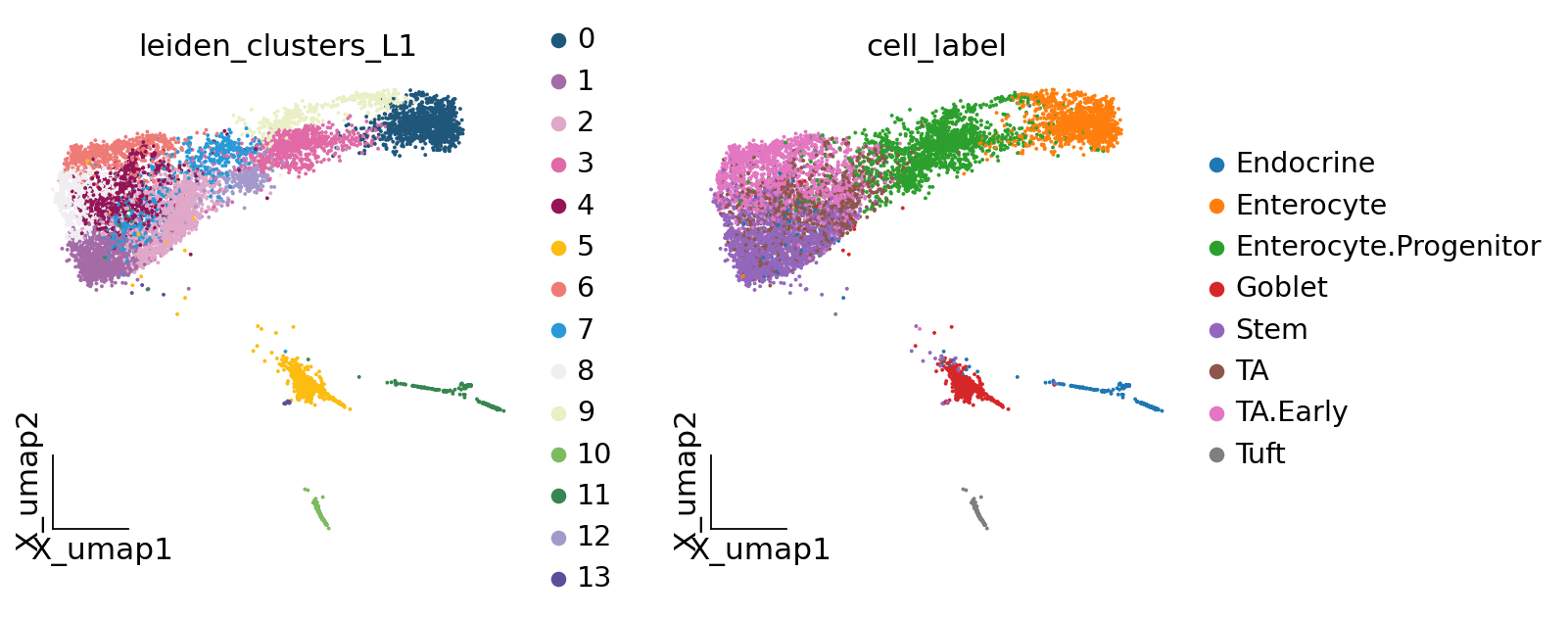
finished: found 14 clusters and added
    'leiden_clusters_L1', the cluster labels (adata.obs, categorical) (0:00:04)
running Louvain clustering
    using the "louvain" package of Traag (2017)
    finished: found 12 clusters and added
    'louvain_clusters_L1', the cluster labels (adata.obs, categorical) (0:00:00)
running Leiden clustering
    finished: found 8 clusters and added
    'leiden_clusters_L2', the cluster labels (adata.obs, categorical) (0:00:02)
running Louvain clustering
    using the "louvain" package of Traag (2017)
    finished: found 8 clusters and added
    'louvain_clusters_L2', the cluster labels (adata.obs, categorical) (0:00:00)
✅ UMAP step already finished, skipping it
✅ tSNE step already finished, skipping it
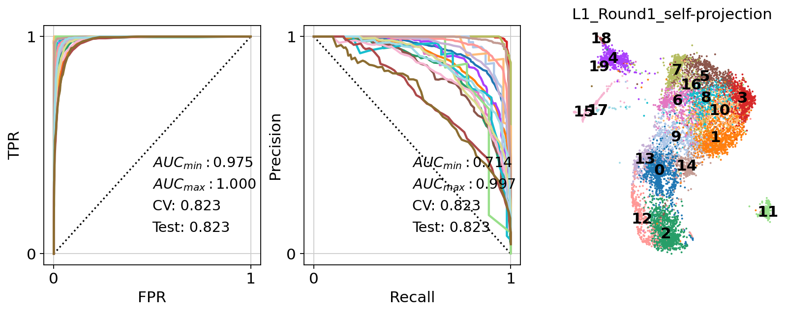
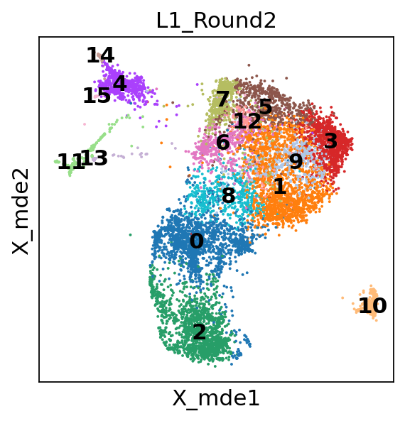
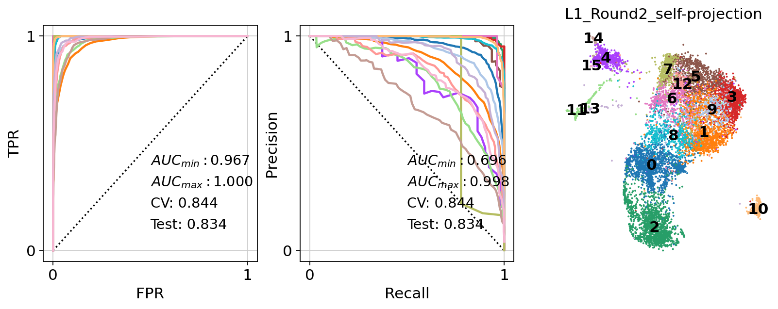
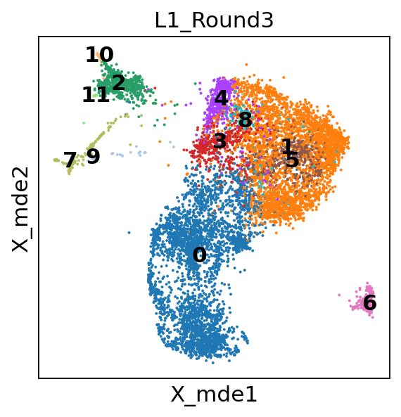
当然,你也可以手动指定参数。这里有一些例子。
adata=ov.single.lazy(
    adata,
    species='mouse',
    reforce_steps=['qc','preprocess','scaled','pca',
                'cell_cycle','Harmony','scVI',
                'eval_bench','umap','tsne'],
    sample_key='batch',
    qc_kwargs={
      'tresh': {'mito_perc': 0.2, 'nUMIs': 500, 'detected_genes': 250},
      'doublets_method': 'scrublet',
      'batch_key': 'batch'
    },
    preprocess_kwargs={
        'mode': 'shiftlog|pearson',
        'n_HVGs': 2000,
        'target_sum': 50*1e4
    },
    pca_kwargs={
        'layer':'scaled',
        'n_pcs':50,
        'use_highly_variable': True,
    },
    harmony_kwargs={
        'n_pcs':50,
    },
    scvi_kwargs={
        'n_layers':2,
        'n_latent':30,
        'gene_likelihood':"nb"
    },
)
ov.plot_set()
ov.pl.embedding(
    adata,
    basis='X_umap',
    color=['leiden_clusters_L1','cell_label']
)
🔬 Starting plot initialization...
🧬 Detecting CUDA devices…
✅ [GPU 0] NVIDIA H100 80GB HBM3
    • Total memory: 79.1 GB
    • Compute capability: 9.0
✅ plot_set complete.
报告生成#
如果你想从lazy函数获得分析报告,这非常简单:运行
omicverse.single.generate_scRNA_report
使用你传递给lazy的相同参数。我们将在未来版本中继续完善报告的布局,我们欢迎你通过GitHub Issues提出建议:Starlitnightly/omicverse#issues
# Usage example:
html_report = ov.single.generate_scRNA_report(
    adata, species='mouse', sample_key='batch',
    output_path="scRNA_analysis_report.html",
)
✅ MultiQC-style report generated successfully!
📄 Report saved to: scRNA_analysis_report.html
📊 Visualizations included: 7 plots
🎨 Features: White theme, Dark mode toggle, OmicVerse logo
🎯 Clustering methods detected: 5
🧬 Integration methods: Harmony ✓, scVI ✓
🏆 Best integration method: X_scVI
<Figure size 640x480 with 0 Axes>
参考文献生成#
从版本1.7.0开始,我们在adata对象中记录了你通过OmicVerse调用的所有包,以方便引用。请注意,此功能仍在开发中,因此某些包可能会缺失。
ov.generate_reference_table(adata)
| method | reference | content | |
|---|---|---|---|
| 0 | SCCAF | clustering optimization with SCCAF | |
| 1 | omicverse | Zeng, Z., Ma, Y., Hu, L., Tan, B., Liu, P., Wa... | This analysis is performed with omicverse fram... |
| 2 | pymde | Agrawal, A., Ali, A., & Boyd, S. (2021). Minim... | MDE with pymde |
| 3 | scanpy | Wolf, F. A., Angerer, P., & Theis, F. J. (2018... | neighbors with scanpy |
| 4 | tsne | Van der Maaten, L., & Hinton, G. (2008). Visua... | t-SNE with omicverse |
| 5 | umap | McInnes, L., Healy, J., & Melville, J. (2018).... | UMAP with pymde |
from IPython.display import IFrame
IFrame(
    src='https://starlitnightly.github.io/single/scRNA_analysis_report.html',
    width=1280,
    height=1000,
)