空间同深度计算

GASTON 是一个可解释的深度学习模型，用于学习基因表达的空间深度。它可以从空间转录组学数据中识别空间依赖的基因表达模式。

import omicverse as ov
# print(f"OmicVerse version: {ov.__version__}")
import scanpy as sc
# print(f"scanpy version: {单细胞.__version__}")
import pandas as pd
import numpy as np

Warning: Could not read dependencies from pyproject.toml: [Errno 2] No such file or directory: '/home/groups/xiaojie/steorra/env/omicverse/lib/python3.10/site-packages/omicverse/pyproject.toml'

   ____            _     _    __                  
  / __ \____ ___  (_)___| |  / /__  _____________ 
 / / / / __ `__ \/ / ___/ | / / _ \/ ___/ ___/ _ \ 
/ /_/ / / / / / / / /__ | |/ /  __/ /  (__  )  __/ 
\____/_/ /_/ /_/_/\___/ |___/\___/_/  /____/\___/                                              

Version: 1.6.11, Tutorials: https://omicverse.readthedocs.io/

准备的 scRNA-seq

首先让我们从 10X Space Ranger 输出中读取空间 Visium 数据。这里我们使用…

# 加载空间数据
adata = sc.read_visium('data/visium_sample/')
print(f'形状: {adata.shape}')

reading /scratch/users/steorra/analysis/omicverse/omicverse_guide/docs/Tutorials-space/data/V1_Human_Lymph_Node/filtered_feature_bc_matrix.h5
 (0:00:01)

AnnData object with n_obs × n_vars = 4035 × 36601
    obs: 'in_tissue', 'array_row', 'array_col'
    var: 'gene_ids', 'feature_types', 'genome'
    uns: 'spatial'
    obsm: 'spatial'

# 运行 GASTON 分析
result = ov.space.gaston(adata)
print('分析完成')

# 可视化
sc.pl.spatial(adata, color=['gaston_depth'], cmap='viridis')

[<AxesSubplot: xlabel='spatial1', ylabel='spatial2'>]

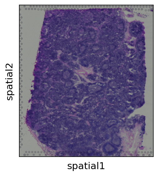
Use top PCs 的 analytic Pearson residualsHere we 计算 PCA 在 analytic Pearson residuals following 该 Scanpy 教程 https://scanpy-tutorials.readthedocs.io/en/latest/tutorial_pearson_residuals.html 教程 . 此 is faster than GLM-PCA, but 该 PCs are 的 lower 质量, so it is not recommended

gas_obj=ov.space.GASTON(adata)gas_obj.get_gaston_input(get_rgb=True,spot_umi_threshold=50)A=gas_obj.get_top_pearson_residuals(num_dims=8,clip=0.01,n_top_genes=5000,                                 use_RGB=True)

filtered out 1 cells that have less than 50 counts
Adding image layer `img1`
calculating RGB
Calculating features `['summary']` using `1` core(s)
Adding `adata.obsm['features']`
Finish (0:00:30)
extracting highly variable genes
--> added
    'highly_variable', boolean vector (adata.var)
    'highly_variable_rank', float vector (adata.var)
    'highly_variable_nbatches', int vector (adata.var)
    'highly_variable_intersection', boolean vector (adata.var)
    'means', float vector (adata.var)
    'variances', float vector (adata.var)
    'residual_variances', float vector (adata.var)
normalizing counts per cell
    finished (0:00:00)
computing analytic Pearson residuals on adata.X
    finished (0:00:00)
computing PCA
    with n_comps=8
    finished (0:00:00)

We first 加载 GLM-PCs 和 coordinates 和 z-score 归一化.

gas_obj.load_rescale(A)

Training 该 GASTON modelNext we train 该 neural network, once 对于 each random initialization.NEURAL NET 参数 (USER CAN CHANGE)architectures are encoded 作为 list, eg [20,20] means two hidden layers 的 大小 20 hidden neurons- isodepth_arch: architecture 对于 isodepth neural network d(x,y) : R^2 -> R - expression_fn_arch: architecture 对于 1-D 表达 函数 h(w) : R -> R^G- num_epochs: number 的 epochs 到 train NN (NOTE: it is sometimes beneficial 到 train longer)- checkpoint: 保存 model after number 的 epochs = multiple 的 checkpoint- out_dir: 文件夹 到 保存 model runs- optimizer:- num_restarts=20

out_dir='/scratch/users/steorra/tmp/tmp'gas_obj.train(    isodepth_arch=[20,20],    expression_fn_arch=[20,20],    num_epochs=5000,    checkpoint=500,    out_dir=out_dir,    optimizer="adam",    num_restarts=20)

VisualizationIf you use 该 model trained above, then 图 will closely match 该 manuscript — but not exactly match — due 到 PyTorch non-determinism 在 seeding (see pytorch/pytorch#7068 ).We also include 该 model used 在 该 paper 对于 reproducibility.

out_dir='/scratch/users/steorra/tmp/tmp'gaston_model, A, S=gas_obj.get_best_model(out_dir=out_dir,                       max_domain_num=8,start_from=2)

best model: /scratch/users/steorra/tmp/tmp/rep9
Kneedle number of domains: 4

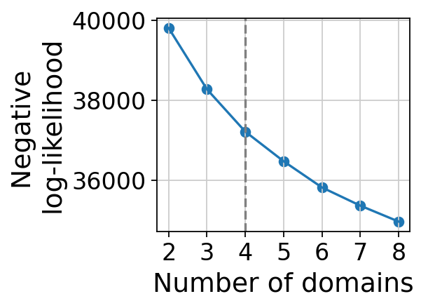
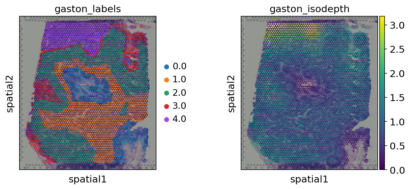
计算 该 IsoDepth 和 LabelsWe can chose 该 number 的 layers 从 IsoDepth

gaston_isodepth, gaston_labels=gas_obj.cal_iso_depth(5)

adata.obs['gaston_labels']=[str(i) for i in gaston_labels]adata.obs['gaston_isodepth']=gaston_isodepth

sc.pl.spatial(adata,             color=['gaston_labels','gaston_isodepth'],             show=False)

[<AxesSubplot: title={'center': 'gaston_labels'}, xlabel='spatial1', ylabel='spatial2'>,
 <AxesSubplot: title={'center': 'gaston_isodepth'}, xlabel='spatial1', ylabel='spatial2'>]

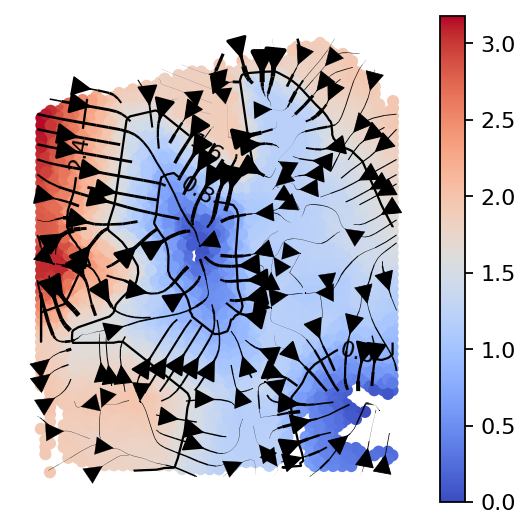
gas_obj.plot_isodepth(show_streamlines=True,                      rotate_angle=-90,arrowsize=2,                      figsize=(4,4),n_neighbors=100)

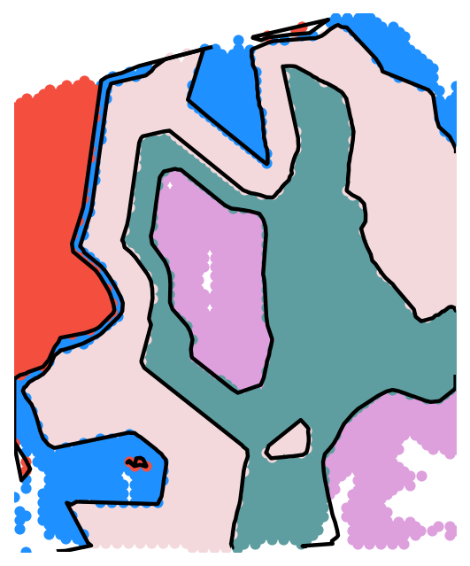
domain_colors=['plum', 'cadetblue', '# F3D9DC','dodgerblue', '#F44E3F']gas_obj.plot_clusters(    domain_colors,    boundary_lw=2,    figsize=(4,5),    rotate_angle=-90,)

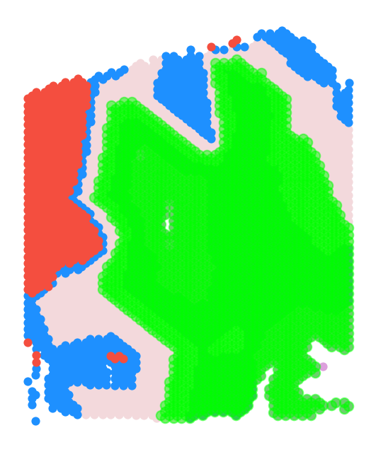
Specific 到 此 analysis: restrict 到 domains (0,1)到 isolate 该 tumor section, we restrict 到 点位 使用 isodepth lying 在 a given range. 该 range 的 isodepth values will need 到 be tuned depending 在 该 specific application.在 some cases, 该 tissue geometry cannot be represented 使用 a single isodepth. 在 此 case, we recommend first subsetting your tissue 到 该 specific region 的 interest (eg 从 ScanPy 聚类分析), 和 then running GASTON

gas_obj.plot_clusters_restrict(    domain_colors,    isodepth_min=0,    isodepth_max=1.5,    rotate_angle=-90,    s=20,lgd=False,    figsize=(4,5))

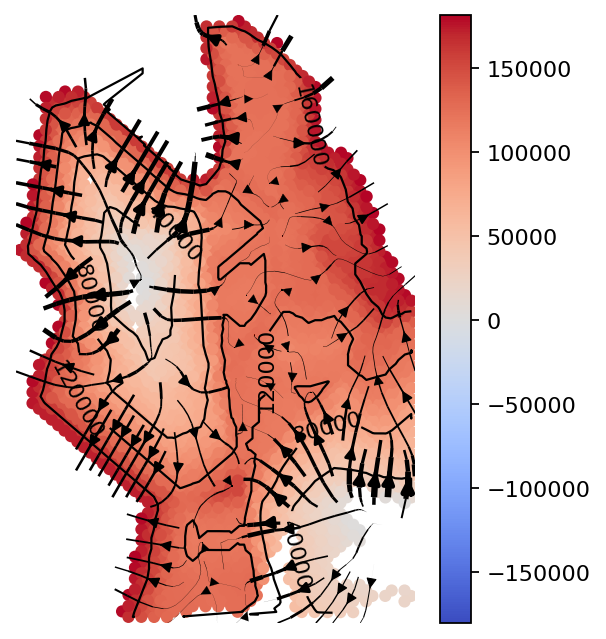
counts_mat_restrict, coords_mat_restrict, gaston_isodepth_restrict, gaston_labels_restrict, S_restrict=gas_obj.restrict_spot(    isodepth_min=0,    isodepth_max=1.5,    adjust_physical=True,    scale_factor=100,    plotisodepth=True,    show_streamlines=True,    rotate_angle=-90,    arrowsize=1, figsize=(4,5),     neg_gradient=True,    n_neighbors=500)

restricting to 2280 spots

gas_obj.filter_genes(    umi_thresh = 1000,    exclude_prefix=['MT-', 'RPL', 'RPS'])

pw_fit_dict=gas_obj.pw_linear_fit()binning_output=gas_obj.bin_data(    num_bins=15,    q_discont=0.95,    q_cont=0.8)

该 binning_output, cont_genes_layer 和 discont_genes_layer stored 在 gas_obj

ad=gas_obj.get_restricted_adata(gas_obj,offset=10**6)

绘制 discontinuous 和 continuous genesWe can found 该 discontinuous 基因 using gas_obj.discont_genes_layer 和 found continuous 基因 using gas_obj.cont_genes_layer

dict(gas_obj.cont_genes_layer)['MARCO']

[0, 2]

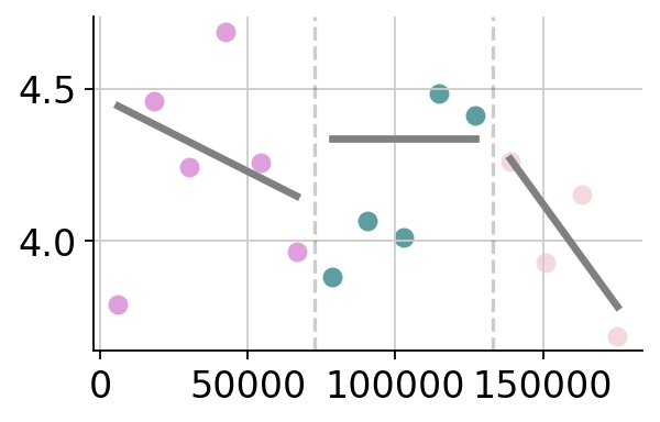
gene='MARCO'gas_obj.plot_gene_pwlinear(gene,domain_colors,offset=10**6,                           cell_type_list=None,pt_size=50,linear_fit=True,                           ticksize=15, figsize=(4,2.5),                           lw=3,domain_boundary_plotting=True)

gene MARCO: discontinuous jump after domain(s) []
gene MARCO: continuous gradient in domain(s) [0, 2]

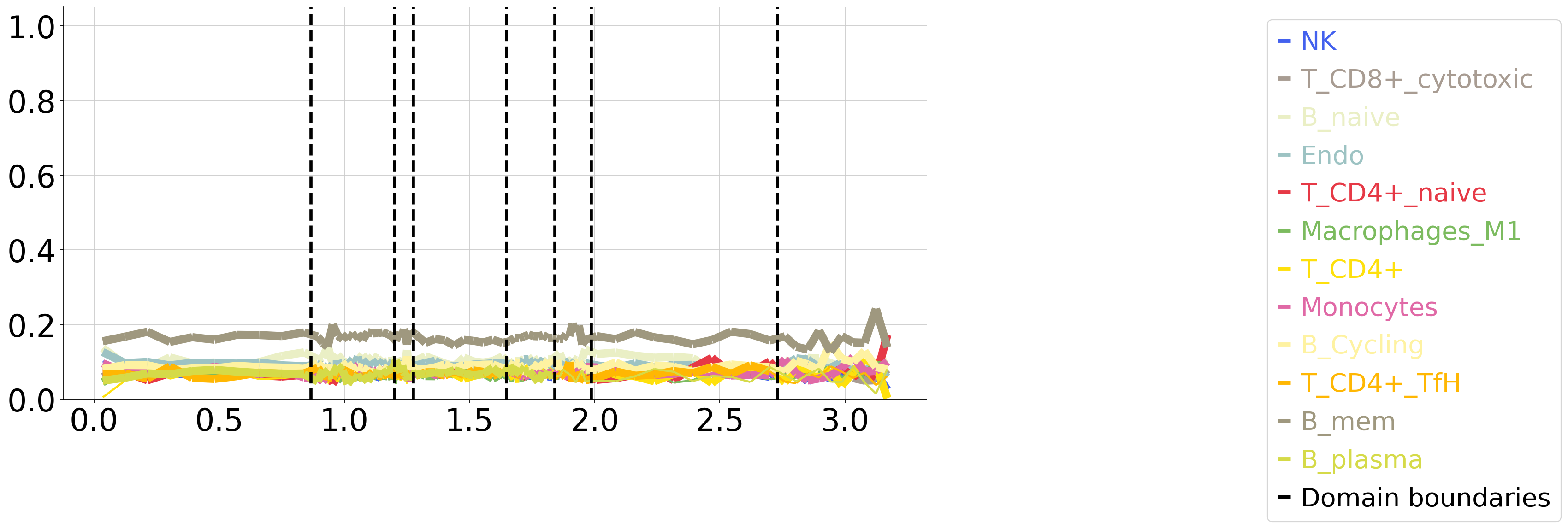
绘制 细胞类型 vs isodepth (如果 细胞类型 info available)加载 细胞类型 标签 per 点位 (从 Tangram). 该 教程 和 result could be found 在 https://omicverse.readthedocs.io/en/latest/Tutorials-space/t_mapping/We store 作为 N x C 数据框 M where M[i,c]=1 如果 点位 i is 细胞类型 c, 和 0 如果 not

cell_type_df=ov.pd.read_csv('data/V1_Human_Lymph_Node_celltype.csv', index_col=0)cell_type_df.head()

	Macrophages_M1	B_IFN	B_GC_LZ	Mast	B_activated	B_GC_DZ	B_mem	T_CD8+_naive	FDC	B_GC_prePB	...	Endo	T_CD8+_cytotoxic	T_CD4+	B_Cycling	T_CD4+_naive	ILC	T_CD4+_TfH	T_CD8+_CD161+	NKT	NK
AAACAAGTATCTCCCA-1	0.082171	0.000017	0.021260	0.000019	0.259048	0.030650	0.504739	0.411314	0.000519	0.000018	...	0.376284	0.043815	0.127287	0.233432	0.006444	0.064583	0.354094	0.170322	0.022457	0.199254
AAACAATCTACTAGCA-1	0.105147	0.000004	0.087364	0.000134	0.009732	0.005403	0.205373	0.039582	0.110013	0.000051	...	0.149988	0.154454	0.160099	0.229329	0.703887	0.057109	0.412450	0.003166	0.053408	0.010387
AAACACCAATAACTGC-1	0.112886	0.000004	0.023793	0.000220	0.228582	0.001881	0.536273	0.156701	0.001156	0.000022	...	0.326906	0.183677	0.110817	0.252126	0.018042	0.083709	0.134888	0.281477	0.001987	0.273480
AAACAGAGCGACTCCT-1	0.150097	0.920552	0.083713	0.089123	0.002341	0.031755	0.321248	0.003961	0.169535	0.000032	...	0.176462	0.398296	0.003631	0.270192	0.353399	0.026902	0.025387	0.015009	0.023835	0.170472
AAACAGCTTTCAGAAG-1	0.281063	0.000003	0.103263	0.000018	0.005834	0.055721	0.433569	0.025195	0.104654	0.000014	...	0.066358	0.032739	0.019467	0.076862	0.072655	0.002734	0.210401	0.037577	0.003070	0.251124

5 rows × 34 columns

from omicverse.external.gaston import plot_cell_typesct_colors=dict(zip(    cell_type_df.columns,    ov.pl.sc_color+ov.utils._plot.palette_28))num_bins_per_domain=[10]*len(set(adata.obs['gaston_labels']))plot_cell_types.plot_ct_props(    cell_type_df,     gaston_labels,     gaston_isodepth,     num_bins_per_domain=num_bins_per_domain,     ct_colors=ct_colors,     ct_pseudocounts={3:1},    include_lgd=True,     figsize=(15,7),    ticksize=30,     width1=8,     width2=2,     domain_ct_threshold=0.5)