STFlow — per-slide flow-matching denoiser

STFlow (Huang et al., ICML 2025 Spotlight) models the joint distribution of gene expression across an entire slide with a spatial transformer + flow-matching denoiser. The training set is the user’s own paired Visium reference; the trained denoiser then runs reverse-time ODE integration on the query tiles’ features + coordinates to sample cohesive whole-slide expression patterns.

Upstream ships training scripts only — there is no released zero-shot checkpoint. (The same group’s productionised successor, STPath, is the zero-shot path; see the STPath tutorial.) This wrapper therefore runs the canonical fit-on-your-reference, predict-on-your-query workflow on a single GPU in 5–10 min.

When to pick STFlow over the alternatives

Goal	Use
Zero-shot prediction on H&E only	stpath
Per-slide fine-tune with paired Visium reference, joint cross-spot modelling	stflow — this notebook
Per-slide fine-tune with paired Visium reference, fast linear baseline	hest_fm
Sub-spot super-resolution on paired Visium+H&E	istar

Environment

import warnings
warnings.filterwarnings('ignore')

import omicverse as ov
import lazyslide as zs
ov.utils.ov_plot_set()

print('omicverse', ov.__version__, '| lazyslide', zs.__version__)

🔬 Starting plot initialization...
🧬 Detecting GPU devices…
✅ NVIDIA CUDA GPUs detected: 1
    • [CUDA 0] NVIDIA H100 80GB HBM3
      Memory: 79.1 GB | Compute: 9.0

   ____            _     _    __                  
  / __ \____ ___  (_)___| |  / /__  _____________ 
 / / / / __ `__ \/ / ___/ | / / _ \/ ___/ ___/ _ \ 
/ /_/ / / / / / / / /__ | |/ /  __/ /  (__  )  __/ 
\____/_/ /_/ /_/_/\___/ |___/\___/_/  /____/\___/                                              

🔖 Version: 2.2.1rc1   📚 Tutorials: https://omicverse.readthedocs.io/
✅ plot_set complete.

omicverse 2.2.1rc1 | lazyslide 0.9.2

How the WSI flows through LazySlide

ov.space.histo wraps LazySlide for tiling, FM embedding, and the WSIData container. STFlow only adds the flow-matching denoiser on top:

omicverse call	LazySlide / wsidata under the hood
ov.space.histo.open_wsi(path) / read_visium_with_image	wsidata.open_wsi → WSIData (a SpatialData subclass)
ov.space.histo.tile(wsi, …)	zs.pp.find_tissues + zs.pp.tile_tissues → wsi.shapes['tiles']
ov.space.histo.embed(wsi, model='ctranspath')	zs.tl.feature_extraction(model='ctranspath') → wsi.tables['ctranspath_tiles']
ov.space.histo.predict_expression(wsi, method='stflow', reference=…)	omicverse-specific: trains the STFlow denoiser on a tile-grid cut from the reference, runs reverse-time ODE on query tile features, writes wsi.tables['stflow_tiles']

Inputs STFlow expects

Same shape as HEST-FM — STFlow trains on the reference slide and predicts on the query tiles:

• reference — paired Visium AnnData with .X, .obsm['spatial'], and uns['spatial'][lib]['scalefactors']['spot_diameter_fullres'].

• wsi — wsidata.WSIData wrapping the H&E. The query tiles are whatever you’ve added via ov.space.histo.tile(); the reference patches are cut out one-per-spot on the same WSI.

• FM features for both reference and query tiles, in wsi.tables['{fm_backbone}_tiles']. STFlow accepts any backbone (768-d CTransPath, 1280-d Virchow2, 1536-d GigaPath / UNI2, …) — feature dimensionality is read from the table; only consistency between reference and query matters.

For your own data:

adata, wsi = ov.space.histo.read_visium_with_image(
    visium_path='/path/to/spaceranger/outs',
    image_path='/path/to/HE.tif',
)

Model weights & cache layout

STFlow has no released pretrained checkpoint (the authors productionised that path as STPath). It is trained from scratch on the user’s paired reference slide every run. The only thing downloaded is the patch encoder.

What	From	To	Size	Gated?
ctranspath patch encoder (default)	LazySlide model registry → HF RendeiroLab/LazySlide-models-gpl	$HF_HOME/hub/ (default ~/.cache/huggingface/hub)	~100 MB	no
STFlow python package	git clone Graph-and-Geometric-Learning/STFlow	$OV_HISTO_CACHE/STFlow/ (added to sys.path automatically)	~80 MB	no
reference / query tile features	computed once	$OV_HISTO_CACHE/ref_features/ and $OV_HISTO_CACHE/tile_features/	~10–50 MB each	—
per-slide denoiser weights	trained each run	in-memory, not persisted	—	—

$OV_HISTO_CACHE defaults to ~/.cache/omicverse/histo; override with OV_HISTO_CACHE=/some/path (recommended on HPC: point it at scratch). $HF_HOME defaults to ~/.cache/huggingface; override with HF_HOME=/some/path.

On first import omicverse also applies a tiny patch to upstream stflow/model/transformer.py (the upstream GeneUpdate.__init__ doesn’t accept a non_negative= kwarg that the caller passes — a known upstream bug). This keeps subsequent re-clones idempotent.

Swapping to a gated backbone — set fm_backbone='uni2' / 'gigapath' / 'virchow2' once you have HuggingFace access. Quality usually improves; training time is unchanged.

Load the demo dataset and tile / embed

This tutorial uses CTransPath (768-d, all-public) so it runs without HuggingFace gating. Swap in 'gigapath', 'uni2', or 'virchow2' for higher accuracy once you have access.

adata, wsi = ov.space.histo.load_breast()
adata

AnnData object with n_obs × n_vars = 3798 × 36601
    obs: 'in_tissue', 'array_row', 'array_col'
    var: 'gene_ids', 'feature_types', 'genome'
    uns: 'spatial', 'histo'
    obsm: 'spatial'

wsi

WSI: /scratch/users/steorra/cache/omicverse_histo/he_zoo/visium_breast/V1_Breast_Cancer_Block_A_Section_1_image.tif
Reader: tiffslide
Dimensions: 24240×24240 (h×w), 1 Pyramid
Pixel physical size: 0.31 MPP

SpatialData object
└── Images
      └── 'wsi_thumbnail': DataArray[cyx] (3, 2000, 2000)
with coordinate systems:
    ▸ 'global', with elements:
        wsi_thumbnail (Images)

Tile the WSI and extract per-tile CTransPath features. Cached on disk under $OV_HISTO_CACHE/tile_features/ so re-runs return instantly.

ov.space.histo.tile(wsi, tile_px=224, mpp=0.5)
ov.space.histo.embed(wsi, model='ctranspath',
                     batch_size=16, num_workers=0)
print('tiles:', len(wsi.shapes['tiles']),
      '| feature table:', list(wsi.tables))

tiles: 1426 | feature table: ['ctranspath_tiles']

Train STFlow on the reference, predict on the query

predict_expression(method='stflow', …) does the following:

1. on first use, auto-clones the upstream STFlow repo into $OV_HISTO_CACHE/STFlow/ and adds it to sys.path,

2. picks n_top_genes HVGs on the reference (or uses the panel you pass via genes=),

3. builds a small spatial-transformer denoiser, sized by n_layers / hidden_dim / n_neighbors,

4. trains it for n_epochs iterations with AdamW on the reference (one forward pass = the whole slide; very cheap per epoch),

5. runs n_sample_steps Euler integration steps of the reverse-time ODE on the query tiles to draw a sample from the conditional distribution p(expression | image, coords),

6. wraps predictions as wsi.tables['stflow_tiles'].

Key parameters

• reference — paired Visium AnnData (required).

• fm_backbone='ctranspath' — any registered pathology FM.

• genes=None — explicit panel; defaults to top-500 HVGs.

• n_epochs=80 — training iterations. The paper trains for thousands of epochs over a multi-slide cohort; 80 is a practical demo budget that still gives meaningful predictions.

• n_layers=4 — depth of the spatial transformer denoiser.

• n_neighbors=8 — number of spatial neighbours each tile attends to.

• n_sample_steps=5 — Euler steps for the reverse-time ODE (paper default).

• hidden_dim=256, batch_size=1 — denoiser sizing.

Gene panel size is fixed at 50 — STFlow’s upstream transformer (stflow/model/transformer.py:63) hardcodes a +50 term in the attention-MLP input dim, so the panel must be exactly 50 genes. Leave genes=None to use the top-50 HVGs from the reference, or pass an explicit 50-gene list.

Pre-staging the patch-encoder weights

STFlow has no released checkpoint of its own (it trains per-slide); the only thing downloaded is the patch encoder you choose via fm_backbone. To run air-gapped or with a vetted local checkpoint:

pred = ov.space.histo.predict_expression(
    wsi, method='stflow', reference=adata,
    fm_backbone='ctranspath',
    fm_weight_path='/scratch/weights/ctranspath.pth',
    cache_dir='/scratch/omicverse_histo',
)

Compute — at the default settings the cell below takes roughly 5–10 min on an H100; most of the time is the ctranspath embed of the reference spot grid (cached for re-runs).

pred = ov.space.histo.predict_expression(
    wsi,
    method='stflow',
    reference=adata,
    fm_backbone='ctranspath',
    n_epochs=80,
    n_layers=4,
    n_neighbors=8,
    n_sample_steps=5,
)
pred

AnnData object with n_obs × n_vars = 1426 × 50
    obs: 'tile_id', 'library_id'
    var: 'gene_ids', 'feature_types', 'genome'
    uns: 'histo'
    obsm: 'spatial'

Reading the output

pred is an AnnData whose rows are query tiles and whose columns are the predicted gene panel:

• pred.X (n_tiles × n_genes) — log1p predicted expression

• pred.var_names — gene symbols (the 500-HVG panel by default, or whatever you passed in genes=)

• pred.obsm['spatial'] — tile pixel centroids

• pred.uns['histo'] — run metadata (method, fm_backbone, n_epochs, n_layers, n_sample_steps).

print('shape       :', pred.shape)
print('first 5 vars:', list(pred.var_names[:5]))
print('coords range:', pred.obsm['spatial'].min(0), '→',
                       pred.obsm['spatial'].max(0))
print('metadata    :', pred.uns['histo'])

shape       : (1426, 50)
first 5 vars: ['ACKR1', 'CFHR1', 'IGKC', 'ANKRD44-IT1', 'ADAMTS9-AS2']
coords range: [4468.5 4355.5] → [22223.5 23521.5]
metadata    : {'method': 'stflow', 'fm_backbone': 'ctranspath', 'n_epochs': 80, 'n_layers': 4, 'n_sample_steps': 5}

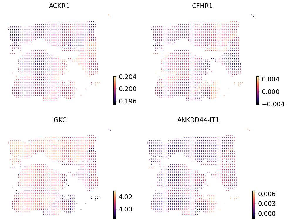
Visualise

ov.pl.embedding(pred, basis='spatial',
                color=list(pred.var_names[:4]),
                cmap='magma', s=12, ncols=2, frameon=False)

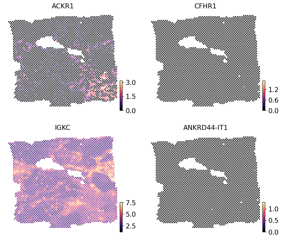
Real Visium counts for the same genes

Plot the same four predicted genes from the paired Visium reference. The reference is log1p-normalised so the colour scale lines up with the STFlow output.

ref = adata.copy()
ov.pp.normalize_total(ref, target_sum=1e4)
ov.pp.log1p(ref)
ov.pl.embedding(ref, basis='spatial',
                color=list(pred.var_names[:4]),
                cmap='magma', s=24, ncols=2, frameon=False)

🔍 Count Normalization:
   Target sum: 10000.0
   Exclude highly expressed: False

✅ Count Normalization Completed Successfully!
   ✓ Processed: 3,798 cells × 36,601 genes
   ✓ Runtime: 0.05s

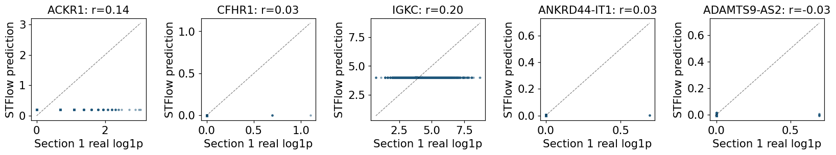
Per-gene scatter on Section 1 (training fit quality)

The Denoiser was trained on Section 1’s spots, so this scatter is the best-case fit. Match each Visium spot to its nearest predicted tile and scatter the real log1p expression against the prediction. Pearson r in the title.

import numpy as np, matplotlib.pyplot as plt
from scipy.spatial import cKDTree
from scipy.stats import pearsonr

spot_xy = adata.obsm['spatial']
tile_xy = pred.obsm['spatial']
nn = cKDTree(tile_xy).query(spot_xy, k=1)[1]

picks = list(pred.var_names[:5])
ref_X = adata[:, picks].X
ref_X = np.log1p(ref_X.toarray() if hasattr(ref_X, 'toarray') else ref_X)
pred_X = pred[:, picks].X[nn]

fig, axes = plt.subplots(1, len(picks), figsize=(3 * len(picks), 3))
for ax, g, i in zip(axes, picks, range(len(picks))):
    ax.scatter(ref_X[:, i], pred_X[:, i], s=4, alpha=0.4)
    r, _ = pearsonr(ref_X[:, i], pred_X[:, i])
    lo = float(min(ref_X[:, i].min(), pred_X[:, i].min()))
    hi = float(max(ref_X[:, i].max(), pred_X[:, i].max()))
    ax.plot([lo, hi], [lo, hi], 'k--', lw=0.8, alpha=0.5)
    ax.set_title(f'{g}: r={r:.2f}')
    ax.set_xlabel('Section 1 real log1p')
    ax.set_ylabel('STFlow prediction')
plt.tight_layout()

Held-out evaluation on a fresh slide (Section 2)

The STFlow Denoiser above was trained on Section 1’s spots and predicts on Section 1’s tiles — its training and query domains overlap, which inflates apparent quality. To get an honest read, predict on Section 2: the adjacent physical section of the same patient block (separate Visium dataset from 10x). Same anatomy and staining batch, but every H&E pixel is new to the trained head.

load_breast(section=2) downloads it on first use (~1.7 GB cached). Note: STFlow’s per-slide head has to be re-trained for the new slide, because the architecture references each slide’s local spot graph during training — we just keep using the same predict_expression(method= 'stflow', reference=adata, ...) call but point wsi= at Section 2 and reference= at Section 1’s spots that we still want to learn from.

adata_s2, wsi_s2 = ov.space.histo.load_breast(section=2)
ov.space.histo.tile(wsi_s2, tile_px=224, mpp=0.5)
ov.space.histo.embed(wsi_s2, model='ctranspath',
                     batch_size=16, num_workers=0)
pred_s2 = ov.space.histo.predict_expression(
    wsi_s2,                       # query: Section 2 H&E tiles
    method='stflow',
    reference=adata,              # train: Section 1 Visium spots
    fm_backbone='ctranspath',
    n_epochs=80, n_layers=4, n_sample_steps=5,
)
pred_s2

AnnData object with n_obs × n_vars = 1857 × 50
    obs: 'tile_id', 'library_id'
    var: 'gene_ids', 'feature_types', 'genome'
    uns: 'histo'
    obsm: 'spatial'

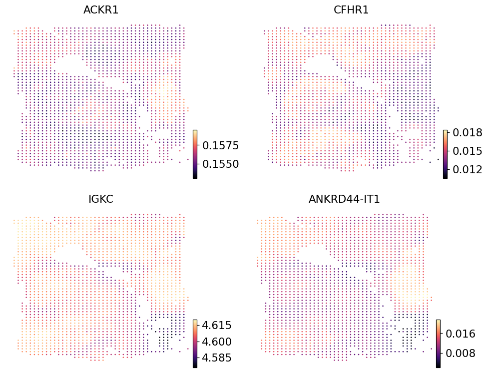
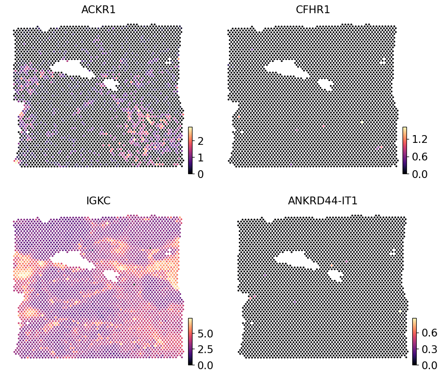
Spatial visualisation on Section 2 — prediction

Same plotter as Section 1, pointed at the held-out slide’s predicted AnnData.

ov.pl.embedding(pred_s2, basis='spatial',
                color=list(pred_s2.var_names[:4]),
                cmap='magma', s=12, ncols=2, frameon=False)

Spatial visualisation on Section 2 — real Visium counts

Section 2’s real Visium expression for the same panel, log1p-normalised.

ref_s2 = adata_s2.copy()
ov.pp.normalize_total(ref_s2, target_sum=1e4)
ov.pp.log1p(ref_s2)
ov.pl.embedding(ref_s2, basis='spatial',
                color=list(pred_s2.var_names[:4]),
                cmap='magma', s=24, ncols=2, frameon=False)

🔍 Count Normalization:
   Target sum: 10000.0
   Exclude highly expressed: False

✅ Count Normalization Completed Successfully!
   ✓ Processed: 3,987 cells × 36,601 genes
   ✓ Runtime: 0.06s

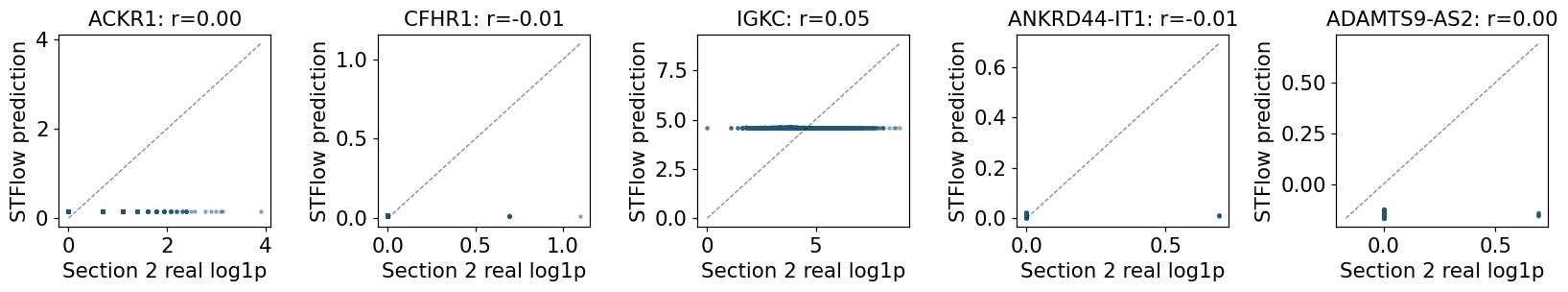
Per-gene scatter on Section 2 (held-out)

Match each Section 2 Visium spot to its nearest Section 2 predicted tile and scatter the real log1p expression against the prediction. Pearson r in the title.

import numpy as np, matplotlib.pyplot as plt
from scipy.spatial import cKDTree
from scipy.stats import pearsonr

spot_xy = adata_s2.obsm['spatial']
tile_xy = pred_s2.obsm['spatial']
nn = cKDTree(tile_xy).query(spot_xy, k=1)[1]

picks = list(pred_s2.var_names[:5])
ref_X = adata_s2[:, picks].X
ref_X = np.log1p(ref_X.toarray() if hasattr(ref_X, 'toarray') else ref_X)
pred_X = pred_s2[:, picks].X[nn]

fig, axes = plt.subplots(1, len(picks), figsize=(3 * len(picks), 3))
for ax, g, i in zip(axes, picks, range(len(picks))):
    ax.scatter(ref_X[:, i], pred_X[:, i], s=4, alpha=0.4)
    r, _ = pearsonr(ref_X[:, i], pred_X[:, i])
    lo = float(min(ref_X[:, i].min(), pred_X[:, i].min()))
    hi = float(max(ref_X[:, i].max(), pred_X[:, i].max()))
    ax.plot([lo, hi], [lo, hi], 'k--', lw=0.8, alpha=0.5)
    ax.set_title(f'{g}: r={r:.2f}')
    ax.set_xlabel('Section 2 real log1p')
    ax.set_ylabel('STFlow prediction')
plt.tight_layout()

Where to go next

Just like the other HE-zoo backends, the predicted AnnData slots straight into ov.space.pySTAGATE, ov.space.svg, and friends. For a head-to-head on the same H&E, see STPath, HEST-FM, and iStar.