Single-cell TCR + transcriptome — the immune-repertoire pipeline

This is the flagship ov.airr single-cell tutorial. It walks the complete workflow for a paired single-cell TCR-seq + gene-expression experiment on a real published dataset, and — as importantly — explains why each step is done the way it is.

Why paired single-cell immune-repertoire data

A T cell carries two identities at once. Its transcriptome says what state it is in — naive, effector, exhausted, regulatory. Its T-cell receptor (TCR) says what clone it belongs to: the receptor is assembled once by V(D)J recombination and then copied unchanged into every daughter cell, so all the descendants of one activated T cell share an identical receptor. The receptor is a natural lineage barcode.

10x 5’-end single-cell sequencing reads both from the same cell:

• a gene-expression (GEX) library — the transcriptome, in adata.X;

• a V(D)J (TCR) library — the rearranged receptor contigs.

Crossing the two answers the question bulk data cannot: which transcriptional states are clonally expanded? A clone that has been driven to proliferate by antigen will appear as many cells sharing one receptor — and if those cells also share a transcriptional state, that state is the one responding to antigen.

The dataset — Wu et al., Nature 2020

We use the tumour-infiltrating T-cell atlas of Wu et al. 2020 (Nature 580:257, PMID 32103181). The study profiled T cells from 14 cancer patients (lung, kidney, colorectal, endometrial) with 10x 5’ scRNA-seq + paired scTCR-seq, sampling three compartments per patient:

• Tumor — the tumour itself;

• NAT — normal adjacent tissue;

• Blood — peripheral blood.

Its central finding: tumour-reactive, clonally expanded T cells are concentrated in exhausted / effector CD8 states inside the tumour — and clonotype sharing reveals movement of clones between blood, normal tissue and tumour. This tutorial reproduces the backbone of that analysis with ov.airr.

The pipeline

load → bridge obsm['airr'] → chain QC → clonotype definition
     → clonal expansion → clonotype network → diversity & overlap
     → V(D)J usage → repertoire x transcriptome

Every stage is one ov.airr call — the same registered, dispatch-based design as ov.protein and ov.es.

0. Setup

ov.airr is the immune-repertoire suite of omicverse. Its single-cell side is AnnData-native: the gene-expression matrix stays in adata.X and the per-cell receptor data lives in adata.obs, so TCR analysis composes directly with the rest of the omicverse single-cell stack via ov.* — no separate object and no external single-cell library needed.

import omicverse as ov
import numpy as np
import pandas as pd
import matplotlib.pyplot as plt
ov.plot_set()

🔬 Starting plot initialization...
🧬 Detecting GPU devices…
✅ NVIDIA CUDA GPUs detected: 1
    • [CUDA 0] NVIDIA H100 80GB HBM3
      Memory: 79.1 GB | Compute: 9.0

   ____            _     _    __                  
  / __ \____ ___  (_)___| |  / /__  _____________ 
 / / / / __ `__ \/ / ___/ | / / _ \/ ___/ ___/ _ \ 
/ /_/ / / / / / / / /__ | |/ /  __/ /  (__  )  __/ 
\____/_/ /_/ /_/_/\___/ |___/\___/_/  /____/\___/                                              

🔖 Version: 2.2.1rc1   📚 Tutorials: https://omicverse.readthedocs.io/
✅ plot_set complete.

1. Load the data

ov.datasets.airr_singlecell() fetches the Wu 2020 atlas as a single AnnData. In a real project you would instead parse your own 10x Cell Ranger V(D)J output with the matching ov.airr reader:

Upstream output	Reader
10x filtered_contig_annotations.csv	ov.airr.read_10x_vdj(...)
10x airr_rearrangement.tsv	ov.airr.read_10x_vdj(...)
AIRR-format rearrangement TSV	ov.airr.read_airr(...)
arbitrary per-contig table	ov.airr.read_tracer(...)

All readers return the same per-cell AIRR layout, so the rest of this pipeline is identical regardless of upstream software.

adata = ov.datasets.airr_singlecell()
print(f"matrix: {adata.n_obs} cells x {adata.n_vars} genes")
print(f"raw counts in .X — max value {adata.X.max():.0f}")
print(f"obs columns : {list(adata.obs.columns)}")
print(f"obsm keys   : {list(adata.obsm.keys())}")

🔍 Downloading data to ./data/wu2020_sctcr.h5ad
⚠️ File ./data/wu2020_sctcr.h5ad already exists
matrix: 5001 cells x 13968 genes
raw counts in .X — max value 9493
obs columns : ['patient', 'sample', 'source', 'cluster_orig', 'cell_type', 'clonotype_orig', 'high_confidence', 'is_cell']
obsm keys   : ['X_umap_orig', 'airr']

The object carries 5001 T cells x 13968 genes. Two pieces of metadata matter for everything below:

• obsm['airr'] — the per-cell TCR contigs, stored as a ragged (variable-length) awkward array: each cell has its own list of receptor chains. This is the scirpy on-disk layout; we bridge it to the ov.airr schema in the next step.

• obsm['X_umap_orig'] — the transcriptome UMAP published with the paper, so we can place every cell in its GEX state without recomputing the embedding.

.obs carries the study design — patient, sample, source (Tumor / NAT / Blood) — and the authors’ transcriptomic annotation in cell_type / cluster_orig (e.g. 8.1-Teff, 8.3a-Trm, 4.3-TCF7).

for c in ["source", "patient"]:
    print(f"--- {c} ---")
    print(adata.obs[c].value_counts())

--- source ---
source
Tumor    2594
NAT      2065
Blood     342
Name: count, dtype: int64
--- patient ---
patient
Lung2     707
Lung3     624
Lung6     619
Lung1     541
Endo1     520
Lung4     455
Renal2    357
Lung5     251
Endo2     203
Endo3     198
Renal1    196
Colon1    154
Renal3    151
Colon2     25
Name: count, dtype: int64

2594 tumour, 2065 normal-adjacent, 342 blood T cells, drawn from 14 patients. That three-compartment, multi-patient design is what lets us ask later whether the tumour repertoire is more clonally focused than blood, and whether clones are shared across tissues.

ov.pl.embedding(adata, basis="X_umap_orig", color="cell_type",
                frameon="small", title="Transcriptome states (Wu 2020)",
                show=False)
plt.show()

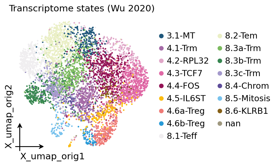
This is the transcriptome view — every dot a T cell, coloured by the authors’ state annotation. The 4.x labels are CD4 states (naive-like 4.3-TCF7, regulatory 4.6-Treg, tissue-resident 4.1-Trm); the 8.x labels are CD8 states (effector 8.1-Teff, tissue-resident memory 8.3a/b/c-Trm, effector-memory 8.2-Tem). The whole tutorial asks: which of these states is clonally expanded? — but to answer it we first need the TCR.

2. Bridge the receptor data into the ov.airr schema

The TCR contigs sit in obsm['airr'] as a ragged array — convenient for storage, awkward for analysis. ov.airr.from_airr_array flattens those contigs and collapses them into a fixed per-cell schema in adata.obs:

• VJ_1 / VJ_2 — the VJ-arm chains (TRA, the TCR alpha chain) — primary and secondary;

• VDJ_1 / VDJ_2 — the VDJ-arm chains (TRB, the TCR beta chain).

Within each arm the chains are ranked by UMI support, so VJ_1 / VDJ_1 are the dominant, most-expressed receptor. The gene-expression matrix and all the original obs metadata are preserved untouched.

adata = ov.airr.from_airr_array(adata)
new_cols = [c for c in adata.obs.columns if c.startswith(("VJ_", "VDJ_"))]
print(f"per-cell AIRR columns added : {len(new_cols)}")
print(f"receptor type per cell:")
print(adata.obs["receptor_type"].value_counts())

per-cell AIRR columns added : 36
receptor type per cell:
receptor_type
TCR          4691
ambiguous     279
no IR          27
BCR             4
Name: count, dtype: int64

Almost every cell carries a TCR, as expected for a sorted T-cell study. A handful are flagged ambiguous (contigs from both TCR and BCR loci — usually ambient contamination) and a few have no IR (no receptor recovered at all). We have not filtered anything yet; we just classified.

3. Chain QC — is the receptor usable?

Not every receptor a droplet reports is biologically plausible. A real T cell has one productive alpha + one productive beta chain. Cell Ranger output deviates from that ideal for two reasons: doublets (two cells in one droplet → too many chains) and dropout (one chain not captured → too few). ov.airr.chain_qc classifies every cell by its chain configuration:

• single pair — one VJ + one VDJ chain. The clean, analysable case.

• orphan VDJ / orphan VJ — only the beta, or only the alpha, recovered. Still usable for clonotype calling (one chain is informative), just less specific.

• multichain — more than two chains in one arm. The hallmark of a doublet; these cells must be excluded — a spurious receptor would create a fake clonotype.

• no IR — no receptor at all.

ov.airr.chain_qc(adata)
print(adata.obs["chain_pairing"].value_counts())
print()
print("receptor subtype:")
print(adata.obs["receptor_subtype"].value_counts().head(3))

chain_pairing
single pair    2593
orphan VDJ     1330
multichain      483
no IR           330
orphan VJ       265
Name: count, dtype: int64

receptor subtype:
receptor_subtype
TRA+TRB      4693
ambiguous     277
no IR          27
Name: count, dtype: int64

The receptor subtype is overwhelmingly TRA+TRB — confirming this is a clean αβ T-cell dataset.

We now build the analysis set: keep cells with a single pair or an orphan chain (all carry a usable receptor for clonotype calling) and drop multichain doublets and no IR cells. This is the central QC decision — every clonotype downstream is only as trustworthy as the receptors that define it.

usable = ["single pair", "orphan VJ", "orphan VDJ"]
tcr = adata[adata.obs["chain_pairing"].isin(usable)].copy()
n_drop = adata.n_obs - tcr.n_obs
print(f"cells with a usable TCR : {tcr.n_obs} / {adata.n_obs}")
print(f"dropped (multichain / no IR): {n_drop}")

cells with a usable TCR : 4188 / 5001
dropped (multichain / no IR): 813

4188 cells carry a usable TCR and form the repertoire we analyse from here on. The dropped ~800 cells are mostly multichain doublets — excluding them before clonotype definition is what keeps the clone calls clean.

4. Clonotype definition

A clonotype is a set of cells that descend from one ancestral T cell — they share an identical receptor. ov.airr offers two definitions, and the difference matters.

define_clonotypes — exact identity. Cells whose primary alpha + beta CDR3 sequences are identical form one clonotype. This is the strict, conservative definition: it counts true clonal descendants. The CDR3 is the hypervariable loop that contacts antigen; identical CDR3s on both chains is overwhelming evidence of a shared ancestor.

ov.airr.define_clonotypes(tcr)
n_clono = tcr.uns["clonotype"]["n_clonotypes"]
print(f"exact clonotypes : {n_clono}")
print(f"largest clone    : {int(tcr.obs['clone_id_size'].max())} cells")
print(f"cells in a clone of size >= 2: "
      f"{int((tcr.obs['clone_id_size'] >= 2).sum())}")

exact clonotypes : 3348
largest clone    : 27 cells
cells in a clone of size >= 2: 1102

define_clonotype_clusters — distance-based. Cells whose CDR3 sequences are merely similar (within a small edit distance) are merged into a clonotype cluster via connected components. This is the looser definition: it captures convergent receptors — independent T cells that recombined near-identical receptors because they recognise the same antigen — and absorbs small sequencing errors. We allow a Hamming distance of 1 (one mismatched residue).

ov.airr.define_clonotype_clusters(tcr, metric="hamming", cutoff=1)
n_clust = tcr.uns["clonotype_clusters"]["n_clusters"]
print(f"exact clonotypes        : {n_clono}")
print(f"distance-based clusters : {n_clust}")

exact clonotypes        : 3348
distance-based clusters : 3331

The cluster count is slightly lower than the exact count: allowing one mismatch merges a few near-identical receptors that strict identity kept apart. The gap is small here because TCRs (unlike hypermutating BCRs) do not somatically mutate — so for the rest of this tutorial we use the exact clone_id, the conservative choice for TCR data.

5. Clonal expansion

define_clonotypes gives every cell a clone size; clonal_expansion turns that continuous size into an interpretable category — 1 (single), 2, 3, >= 4 — so we can ask what fraction of the repertoire is expanded.

ov.airr.clonal_expansion(tcr)
exp = tcr.obs["clonal_expansion"].value_counts()
frac_exp = 100.0 * (tcr.obs["clonal_expansion"] != "1 (single)").mean()
print(exp)
print(f"\ncells in an expanded (>=2) clone: {frac_exp:.1f}%")

clonal_expansion
1 (single)    3010
>= 4           531
2              424
3              147
Name: count, dtype: int64

cells in an expanded (>=2) clone: 28.1%

Roughly a quarter of the cells sit in an expanded clone (size ≥ 2), and a substantial group falls in the >= 4 bucket — large clones that have proliferated extensively. The other three-quarters are singletons: clones seen exactly once. A repertoire that is part highly-expanded, part vast singleton tail is the classic signature of an antigen-experienced T-cell population — a few clones driven to expand against specific antigens, on a background of unexpanded diversity.

ov.airr.clonal_expansion_plot(tcr, groupby="source")
plt.show()

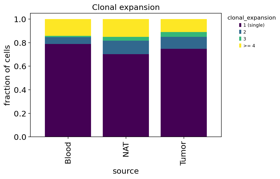
Split by tissue, the expanded fraction is highest in the tumour and lowest in blood — the first hint of the paper’s story: the tumour microenvironment locally drives clonal proliferation. We quantify that rigorously with diversity metrics in section 7.

6. Clonotype network

The clonotype network is a graph view of the repertoire: every cell is a node, and an edge links two cells whose receptors are identical (or, with a cutoff, similar). Connected components are clonotypes; large dense blobs are expanded clones, isolated dots are singletons. clonotype_network computes a 2-D layout and stores it in obsm['X_clonotype_network'].

We set min_cells=2 to hide singletons — with thousands of unique receptors they would swamp the plot — and focus the layout on the expanded clones that carry the biological signal.

ov.airr.clonotype_network(tcr, min_cells=2)
n_comp = tcr.uns["clonotype_network"]["n_components"]
print(f"expanded clonotypes drawn (size >= 2): {n_comp}")

expanded clonotypes drawn (size >= 2): 338

ov.airr.clonotype_network_plot(tcr, color="clonal_expansion",
                               title="Clonotype network (expanded clones)")
plt.show()

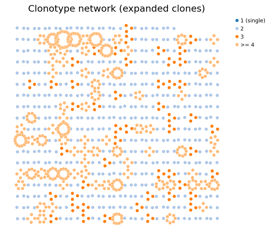
Each ring is one expanded clonotype; ring size scales with clone size. The big rings — coloured by the >= 4 category — are the dominant clones that have proliferated most. This is the repertoire’s clonal skeleton: a few large families standing out from many small ones.

ov.airr.clonotype_network_plot(tcr, color="source",
                               title="Clonotype network by tissue")
plt.show()

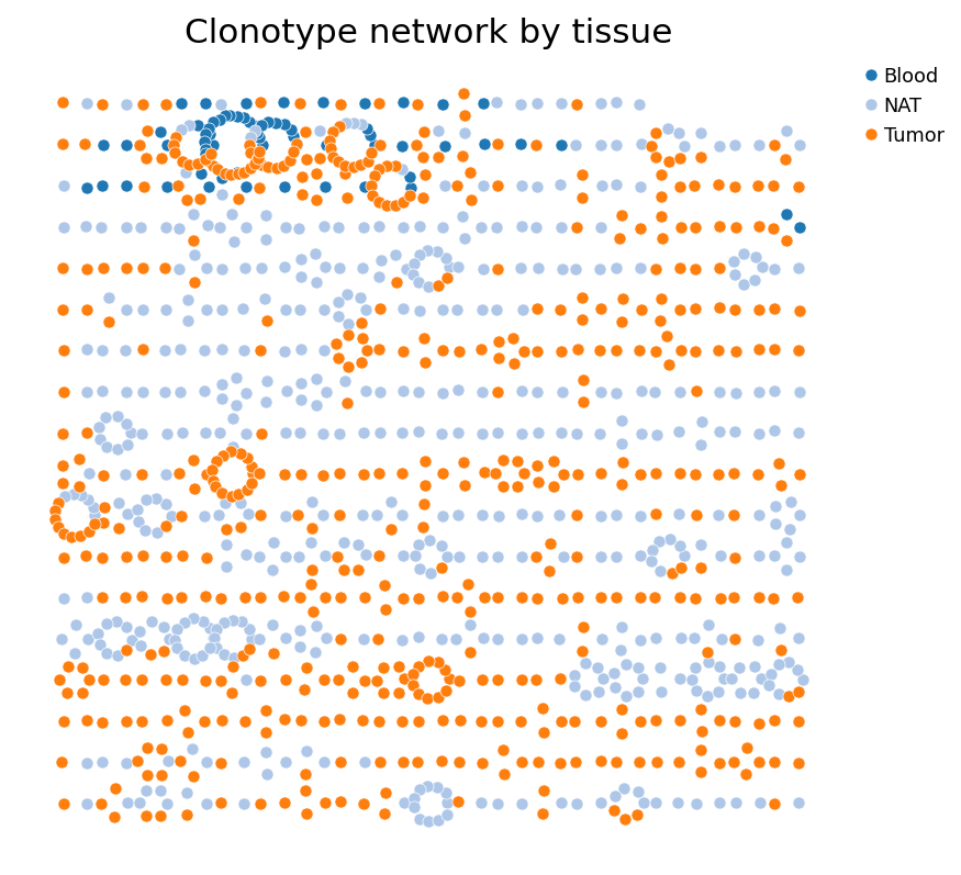
Re-colouring the same layout by tissue is revealing: many rings mix Tumor and NAT (and occasionally Blood) cells. A single clonotype spanning two compartments means one clonal family is present in both — direct evidence that T-cell clones traffic between normal tissue and tumour, exactly the clonal-sharing phenomenon Wu 2020 reported.

7. Repertoire diversity and overlap

Alpha diversity — how clonally focused is each compartment?

A repertoire dominated by a few big clones is less diverse than one of equal size made of many small clones. alpha_diversity quantifies this from the clone-size distribution. We use normalized Shannon entropy (1 = perfectly even, every clone unique; lower = a few clones dominate), computed per tissue.

div = ov.airr.alpha_diversity(tcr, groupby="source",
                              metric="normalized_shannon")
print(div)

n_cells  n_clonotypes  normalized_shannon
group                                           
Blood      307           272            0.975210
NAT       1678          1378            0.980015
Tumor     2127          1818            0.984513

All three values are high — most clones are still singletons everywhere — but the ordering is the biology: diversity is lowest in the tumour and highest in blood. The tumour repertoire is the most clonally focused: a subset of clones has expanded there at the expense of evenness, which is what antigen-driven proliferation inside the tumour produces. Blood, a transit compartment not under local antigen pressure, stays the most even.

summary = ov.airr.alpha_diversity(
    tcr, groupby="source",
    metric=["normalized_shannon", "gini_simpson", "d50"])
summary.round(3)

	n_cells	n_clonotypes	normalized_shannon	gini_simpson	d50
group
Blood	307	272	0.975	0.993	119
NAT	1678	1378	0.980	0.999	539
Tumor	2127	1818	0.985	0.999	755

Three diversity metrics agree. D50 — the number of top clones needed to cover half the cells — is the most intuitive: a smaller D50 means a few clones carry the repertoire. Reading the table by tissue confirms the tumour is the most clonally constricted compartment.

Repertoire overlap — are clonotypes shared between patients?

repertoire_overlap builds a pairwise matrix of how many clonotypes two groups share. Computed across the 14 patients with the Jaccard index, it tests whether clonotypes are private (each patient’s TCRs unique to them) or public (shared).

ov.airr.repertoire_overlap_plot(tcr, groupby="patient", metric="jaccard")
plt.show()

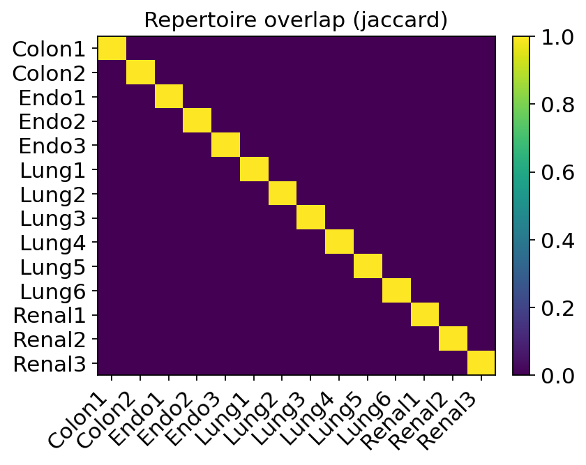
The heatmap is near-zero off the diagonal: almost no clonotype is shared between patients. This is expected and reassuring — an exact-CDR3 clonotype is essentially patient-private, because V(D)J recombination plus each individual’s HLA make the odds of two people independently producing the identical receptor vanishingly small. It also validates the clonotype definition: if unrelated patients did share many clones, we would suspect a barcode or demultiplexing artefact. Clonal expansion here is a within-patient, within-tumour process.

8. V(D)J gene usage

Before recombination, each TCR chain picks one V, (one D,) and one J gene segment from the germline. The frequency with which each segment is used — the gene-usage profile — is a coarse fingerprint of a repertoire; strong skewing can flag a biased or antigen-selected response. vdj_usage tabulates segment frequencies, here for the TRBV (beta-chain V) genes, split by tissue.

ov.airr.vdj_usage_plot(tcr, gene="v", chain="VDJ_1",
                       groupby="source", top=12)
plt.show()

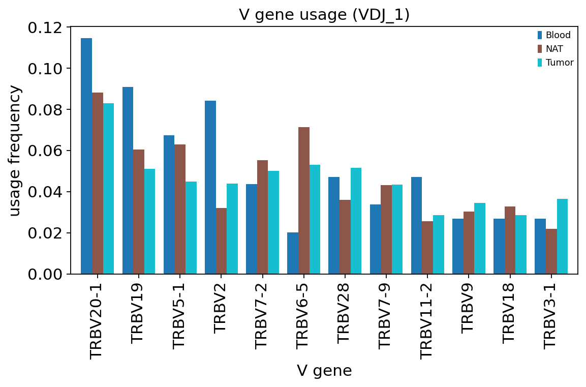
The most-used TRBV segments are common, well-known genes (e.g. TRBV20-1, TRBV28, TRBV9) and their frequencies are broadly similar across Tumor, NAT and Blood. That is the expected result: V-gene usage is set mostly by germline recombination biases, which are shared across a patient’s compartments. The tumour’s clonal focusing seen in section 7 is driven by expansion of particular clones, not by a wholesale shift in which V genes are used — gene usage and clonal expansion are different axes of the repertoire.

9. Repertoire meets transcriptome — the central question

Everything so far used only the TCR. Now we cross it with the GEX annotation in cell_type to answer the question that motivates paired single-cell immune-profiling: which transcriptional states are clonally expanded?

We tabulate, for every transcriptomic state, the fraction of its cells falling in each clonal-expansion category. A state made mostly of singletons is not proliferating; a state rich in large (>= 4) clones is.

ct_exp = ov.airr.clonal_expansion_composition(tcr, groupby="cell_type")
ct_exp.round(3)

clonal_expansion	1 (single)	2	3	>= 4
cell_type
8.1-Teff	0.387	0.134	0.071	0.408
8.3b-Trm	0.469	0.144	0.067	0.321
8.3c-Trm	0.538	0.176	0.061	0.226
8.4-Chrom	0.652	0.087	0.043	0.217
8.2-Tem	0.611	0.152	0.065	0.172
8.3a-Trm	0.663	0.142	0.046	0.149
3.1-MT	0.656	0.138	0.064	0.142
8.5-Mitosis	0.661	0.102	0.102	0.136
4.1-Trm	0.794	0.131	0.025	0.050
4.2-RPL32	0.884	0.061	0.006	0.049
4.4-FOS	0.894	0.068	0.007	0.032
8.6-KLRB1	0.829	0.122	0.024	0.024
4.5-IL6ST	0.918	0.058	0.000	0.023
4.6b-Treg	0.911	0.071	0.000	0.018
4.3-TCF7	0.987	0.007	0.000	0.006
4.6a-Treg	0.958	0.038	0.004	0.000

The table is the punchline of the tutorial. Read the >= 4 column — the fraction of each state’s cells sitting in a large, highly-expanded clone:

• the CD8 effector / tissue-resident-memory states top the list — 8.1-Teff, 8.3b-Trm, 8.3c-Trm, 8.2-Tem. These are the cytotoxic, antigen-experienced, exhaustion-leaning CD8 T cells, and they are by far the most clonally expanded compartment.

• the CD4 naive-like and regulatory states sit at the bottom — 4.3-TCF7 is almost entirely singletons, and the 4.x states generally show little expansion.

This is precisely the Wu 2020 finding: clonal expansion is not spread evenly across T-cell states — it is concentrated in the effector / exhausted CD8 compartment inside the tumour. Those are the tumour-reactive T cells that recognised antigen, proliferated, and now dominate the tumour repertoire.

fig, ax = plt.subplots(figsize=(7, 4.5))
ct_exp.plot(kind="bar", stacked=True, ax=ax, colormap="viridis", width=0.82)
ax.set_ylabel("fraction of cells")
ax.set_xlabel("transcriptomic state")
ax.set_title("Clonal expansion across T-cell states")
ax.legend(title="clonal_expansion", bbox_to_anchor=(1.02, 1),
          loc="upper left", fontsize=8, frameon=False)
plt.show()

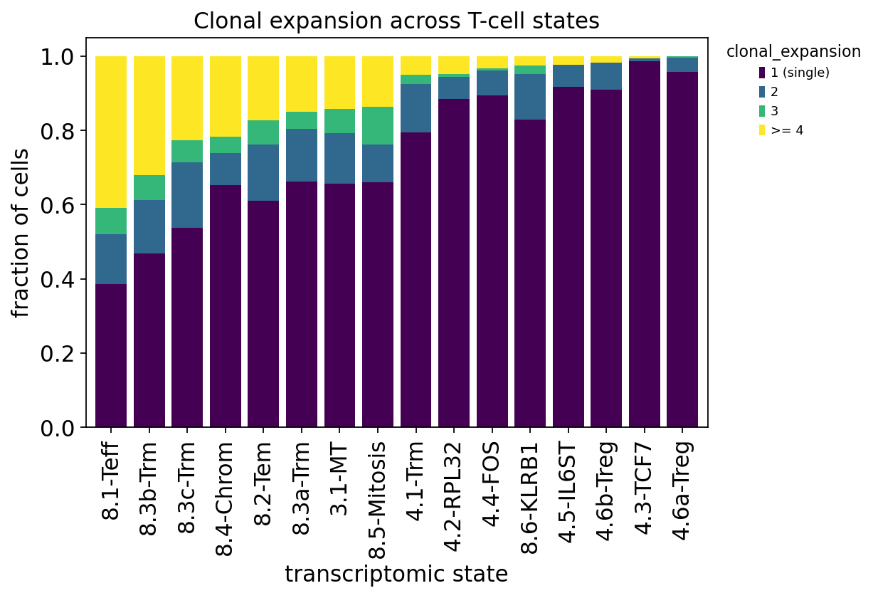
The stacked bars make it visual: the dark 1 (single) block dominates the naive/regulatory CD4 states on the right, while the bright >= 4 band swells in the CD8 effector/Trm states on the left. Transcriptional state and clonal behaviour are coupled — and only paired single-cell data can show it.

We can also project the clonal signal straight onto the transcriptome UMAP: by copying the per-cell clone_id_size from the TCR subset back onto the full object, every cell’s GEX position can be coloured by how expanded its clone is.

adata.obs["clone_size"] = np.nan
adata.obs.loc[tcr.obs_names, "clone_size"] = tcr.obs["clone_id_size"].values
ov.pl.embedding(adata, basis="X_umap_orig", color="clone_size",
                cmap="Reds", frameon="small",
                title="Clone size on the transcriptome UMAP", show=False)
plt.show()

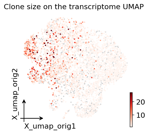
The expanded (red) cells are not scattered at random — they pile up in the CD8 effector / Trm region of the transcriptome, the same neighbourhood that topped the table. The lineage barcode and the cell state tell one coherent story.

10. Innate-like invariant T cells

Not every T cell in a tumour is a conventional, antigen-specific αβ T cell. A minority belong to innate-like lineages whose receptor is semi-invariant — built from an almost-fixed germline V/J combination shared across individuals — so they recognise non-peptide antigens and respond fast, more like innate cells:

• MAIT (mucosal-associated invariant T) cells — a TRAV1-2 alpha chain rearranged to TRAJ33 (or TRAJ12 / TRAJ20); they sense microbial riboflavin metabolites presented on MR1.

• iNKT (invariant natural killer T) cells — a TRAV10/TRAV24 alpha chain rearranged to TRAJ18; they sense lipid antigens on CD1d.

ov.airr.detect_invariant applies those germline-gene rules to the VJ (alpha) chain and writes the call to obs['invariant_tcell']. Spotting these cells matters: their invariant receptors would otherwise be read as ordinary clonotypes, and they behave differently from conventional tumour-reactive T cells.

ov.airr.detect_invariant(tcr)
inv = tcr.obs["invariant_tcell"].value_counts()
n_innate = int(inv.get("MAIT", 0) + inv.get("iNKT", 0))
print(inv)
print(f"\ninnate-like (MAIT + iNKT): {n_innate} cells "
      f"({100.0 * n_innate / tcr.n_obs:.1f}% of the repertoire)")

invariant_tcell
conventional    3002
unknown         1157
MAIT              27
iNKT               2
Name: count, dtype: int64

innate-like (MAIT + iNKT): 29 cells (0.7% of the repertoire)

The repertoire is, as expected for a tumour T-cell atlas, overwhelmingly conventional — a small but real MAIT population is flagged, and only a couple of iNKT cells. The unknown cells are those with no recovered alpha (VJ) chain, so the invariant rule cannot be evaluated — these are the orphan VDJ cells kept at the QC step. The MAIT fraction is the biologically interesting number: MAIT cells are a minor, antigen-non-specific component that should not be mistaken for tumour-reactive expansion.

ax = ov.pl.embedding(adata, basis="X_umap_orig",
                     color="cell_type", frameon="small",
                     title="MAIT / iNKT cells on the transcriptome",
                     show=False)
inv_cells = tcr.obs_names[tcr.obs["invariant_tcell"].isin(["MAIT", "iNKT"])]
xy = adata[inv_cells].obsm["X_umap_orig"]
ax.scatter(xy[:, 0], xy[:, 1], s=22, c="black", marker="D",
           edgecolors="white", linewidths=0.4, zorder=5, label="MAIT/iNKT")
ax.legend(loc="upper right", fontsize=8, frameon=False)
plt.show()

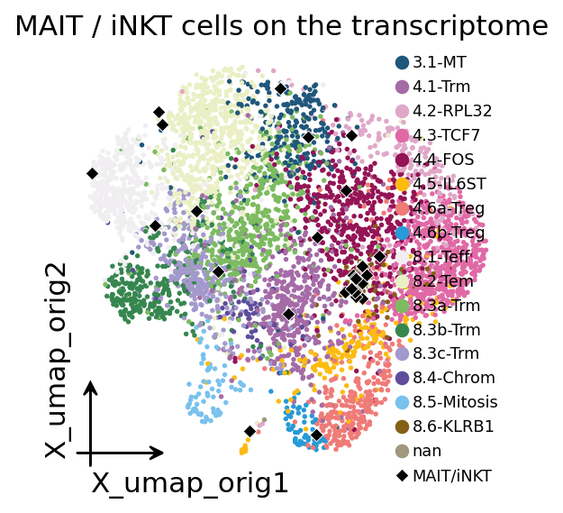
Overlaying the invariant cells (black diamonds) on the transcriptome UMAP shows they are not scattered at random: MAIT cells cluster in a specific corner of the CD8 compartment — consistent with their characteristic effector-memory, KLRB1 (CD161)-high transcriptional program — rather than mixing into the conventional effector/exhausted states that dominate the clonally expanded core. Receptor genetics and transcriptional state agree on which cells are innate-like.

11. Clonotype imbalance between compartments

Section 7 showed the tumour repertoire as a whole is clonally focused. A sharper question is: which individual clonotypes are disproportionately abundant in one compartment versus another? A clone enriched in the tumour relative to blood is a candidate tumour-reactive clone — one that recognised tumour antigen and proliferated in situ.

ov.airr.clonotype_imbalance answers this per clonotype. For each clone it builds a 2x2 contingency table (cells of this clone vs all other cells, in case vs control), runs a Fisher exact test, and reports a log2 fold-change and a BH-corrected p-value. We compare the tumour against blood — the most distinct pair of compartments.

imb = ov.airr.clonotype_imbalance(tcr, groupby="source",
                                  case="Tumor", control="Blood")
print(f"clonotypes tested : {len(imb)}")
print(f"significant (padj < 0.05): {int((imb['pvalue_adj'] < 0.05).sum())}")
imb.head(8).round(3)

clonotypes tested : 2065
significant (padj < 0.05): 1

	clone_id	n_case	n_control	log2_fold_change	pvalue	pvalue_adj
0	clonotype_0	11	16	-3.291	0.000	0.0
1	clonotype_1	9	7	-2.467	0.002	1.0
2	clonotype_39	1	3	-3.788	0.007	1.0
3	clonotype_186	0	2	-4.373	0.016	1.0
4	clonotype_201	0	2	-4.373	0.016	1.0
5	clonotype_190	0	2	-4.373	0.016	1.0
6	clonotype_5	8	4	-1.940	0.054	1.0
7	clonotype_54	2	2	-2.788	0.080	1.0

The table is sorted by raw p-value. Read the log2_fold_change column: positive values mark clones enriched in the tumour, negative values clones enriched in blood. The top hit clears multiple-testing correction — a clone that is genuinely, significantly skewed between the two compartments. Most other clones do not survive BH correction, and that is itself informative: with a few hundred blood cells each individual clone is rare, so only the most extreme imbalances reach significance — the test is appropriately conservative rather than calling every small fluctuation a tumour-reactive clone.

# Take the 8 most blood-enriched + the 7 most tumour-enriched clones,
# ranked by log2 fold-change magnitude — this surfaces both directions
# rather than only the lowest-p (which happen to all be blood-enriched).
blood_side = imb.sort_values('log2_fold_change').head(8)
tumor_side = imb.sort_values('log2_fold_change', ascending=False).head(7)
top_imb = pd.concat([blood_side, tumor_side]).sort_values('log2_fold_change')
colors = ['#d62728' if v > 0 else '#1f77b4'
          for v in top_imb['log2_fold_change']]
fig, ax = plt.subplots(figsize=(6.5, 4.2))
ax.barh(top_imb['clone_id'].astype(str), top_imb['log2_fold_change'],
        color=colors)
ax.axvline(0, color='k', lw=0.8)
ax.set_xlabel('log2 fold-change  (Tumor / Blood)')
ax.set_title('Top imbalanced clonotypes  (blood-enriched / tumor-enriched)')
ax.spines[['top', 'right']].set_visible(False)
plt.tight_layout()
plt.show()

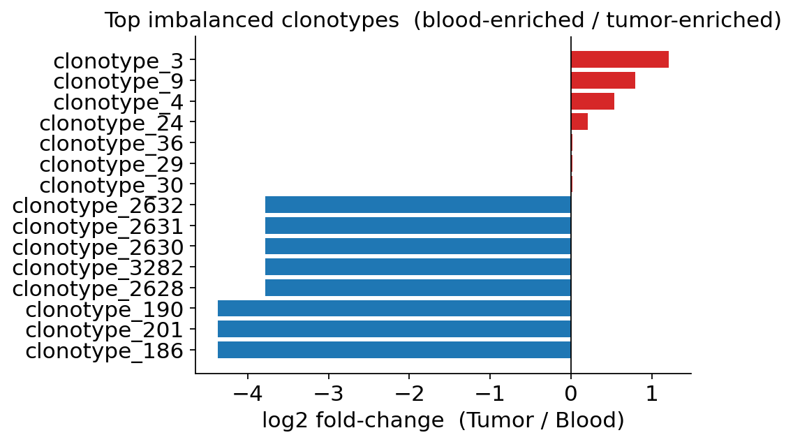
The bar plot makes the direction visible. We forced both sides of the imbalance to be shown — the top 8 blood-enriched (blue, negative log2FC) and the top 7 tumour-enriched (red, positive log2FC). If we had simply taken the lowest p-values (imb.head(15)) we would have seen only blood-enriched clones — because in this 5 k-cell subset blood-skewed clones are the largest and so reach significance most easily.

Read the figure in two halves:

• Blood-enriched clones (top, blue) are the large circulating clonotypes with most of their cells in the blood compartment — memory clones that have expanded systemically and bled out into the periphery.

• Tumour-enriched clones (bottom, red) are clones whose cells sit preferentially in the tumour — candidate tumour-reactive families, even though none individually reaches BH-corrected significance in this small subset (only the very largest blood-enriched clone clears padj < 0.05; the test is conservative when blood has only ~300 cells).

This per-clone view complements the whole-repertoire diversity metrics: diversity tells us the tumour is focused, imbalance tells us which clones drive that focus.

12. Clonotype transcriptional coherence (modularity)

Cells of one clonotype are clonal descendants of a single T cell — but do they all still occupy the same transcriptional state? A clone whose cells are all 8.1-Teff is transcriptionally coherent: it was driven into one fate. A clone scattered across many states has differentiated — its descendants took divergent paths.

ov.airr.clonotype_modularity quantifies this. For each clonotype it reports the largest fraction of its cells sharing one transcriptomic cluster (modularity_score, near 1 = coherent) and which cluster that is (dominant_cluster). We use the authors’ cell_type annotation as the transcriptomic clustering.

mod = ov.airr.clonotype_modularity(tcr, cluster_key="cell_type")
mod_exp = mod[mod["size"] >= 3]
print(f"clonotypes scored        : {len(mod)}")
print(f"expanded (size >= 3)     : {len(mod_exp)}")
print(f"mean modularity (size>=3): {mod_exp['modularity_score'].mean():.3f}")
mod_exp.head(8)

clonotypes scored        : 3348
expanded (size >= 3)     : 126
mean modularity (size>=3): 0.593

	clone_id	size	modularity_score	dominant_cluster
0	clonotype_0	27	0.370370	8.2-Tem
1	clonotype_1	18	0.555556	8.3b-Trm
2	clonotype_2	17	0.294118	8.1-Teff
3	clonotype_3	15	0.533333	8.3c-Trm
4	clonotype_4	15	0.666667	8.2-Tem
5	clonotype_6	14	0.785714	8.1-Teff
6	clonotype_5	14	0.357143	8.1-Teff
7	clonotype_7	12	0.666667	8.1-Teff

The largest clones already show high modularity scores: the cells of a typical expanded clone are mostly confined to one or two transcriptomic states, not spread thinly across all of them. The dominant_cluster column is revealing — the big clones land in CD8 effector / tissue-resident-memory states (8.x), exactly the compartment section 9 flagged as the clonally expanded one.

# Modularity vs size scatter — use the omicverse palette and styling
from omicverse.pl._palette import green_color
fig, ax = plt.subplots(figsize=(6.2, 3.8))
ax.scatter(mod['size'], mod['modularity_score'], s=18,
           alpha=0.55, c=green_color[0], edgecolors='white', linewidths=0.3)
ax.set_xscale('log')
ax.set_xlabel('clone size (cells, log scale)')
ax.set_ylabel('modularity score')
ax.set_title('Transcriptional coherence vs clone size')
ax.spines[['top', 'right']].set_visible(False)
dom = mod_exp['dominant_cluster'].value_counts().head(5)
print('dominant cluster of expanded clones:')
print(dom)
plt.tight_layout()
plt.show()

dominant cluster of expanded clones:
dominant_cluster
8.1-Teff    40
8.2-Tem     24
3.1-MT      16
8.3a-Trm    13
8.3b-Trm    12
Name: count, dtype: int64

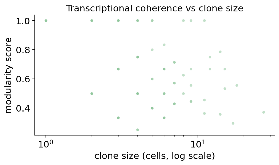
The scatter shows the trade-off: singletons sit at score 1 trivially (one cell is its own cluster), but among genuinely expanded clones the scores stay high — large clones do not dissolve into transcriptional noise. The printed tally confirms the dominant state of expanded clones is overwhelmingly the CD8 effector / Trm compartment. Clonal expansion and transcriptional identity are coupled not just in aggregate (section 9) but clone by clone: a proliferating tumour clone tends to be a coherent block of effector CD8 cells.

13. CDR3 motif logos

The CDR3 loop is the most variable part of the receptor and the part that physically contacts antigen. A sequence logo stacks the per-position amino-acid composition of a set of CDR3s, with letter height scaled to information content (bits): tall, conserved columns are positions fixed across the set, short columns are free to vary.

ov.airr.cdr3_logo draws this. Run on the whole repertoire it shows the generic CDR3 grammar; run on a single expanded clonotype it collapses to that one receptor’s exact sequence — a useful sanity check that the clone really is one receptor. We first show the whole-beta-chain logo.

ax = ov.airr.cdr3_logo(tcr, chain="beta", kind="information")
ax.set_title("CDR3\u03b2 logo \u2014 whole repertoire")
plt.show()

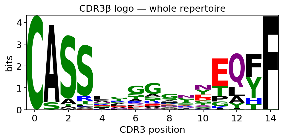
Across thousands of distinct receptors the only tall columns are the conserved CDR3 termini — the near-invariant C … F framework residues that flank every TCR-beta CDR3 — while the central, antigen- contacting positions are low and mixed: the hypervariable core is, as expected, not conserved at the repertoire level.

The motif becomes meaningful when restricted to receptors that share a specificity. We draw the CDR3β logo for the single most expanded clonotype — all its cells are clonal descendants, so they must carry one identical receptor.

top_clone = tcr.obs["clone_id"].value_counts().index[0]
sub = tcr[tcr.obs["clone_id"] == top_clone]
ax = ov.airr.cdr3_logo(sub, chain="beta", kind="information")
ax.set_title(f"CDR3\u03b2 logo \u2014 {top_clone} (n={sub.n_obs} cells)")
plt.show()

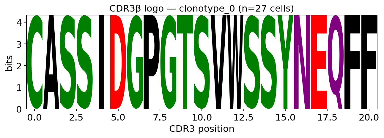
For the expanded clone every position is a single full-height letter: the logo spells out one exact CDR3β sequence. That is the visual definition of a clonotype — many cells, one receptor — and confirms the exact-identity clonotype call from section 4. The same function, run on a distance-based cluster or a specificity_groups motif group, would instead reveal a partly-conserved motif: a shared antigen-binding grammar across convergent receptors.

14. Antigen-specificity annotation against VDJdb

A clonotype tells us cells are clonally related and clonal expansion tells us a clone responded to something — but not to what. The receptor sequence itself carries that information: TCRs of known specificity have been catalogued in public databases. VDJdb is the largest, pairing thousands of CDR3 sequences with their cognate epitope (the exact peptide), source antigen and species.

ov.datasets.vdjdb_reference() ships VDJdb as a DataFrame, and ov.airr.annotate_antigen matches every query TCR’s CDR3 against it (exactly, or within a TCRdist radius) and attaches the best hit’s epitope peptide, source antigen and species. We match the beta chain against the human TRB records by exact CDR3 identity — the conservative setting.

ref = ov.datasets.vdjdb_reference()
ref_trb = ref[ref["gene"] == "TRB"]
print(f"VDJdb TRB reference records : {len(ref_trb)}")
print(f"distinct epitope peptides   : {ref_trb['antigen_epitope'].nunique()}")
print(f"distinct source antigens    : {ref_trb['antigen_gene'].nunique()}")
print(ref_trb["antigen_species"].value_counts().head(6))

🔍 Downloading data to ./data/vdjdb_reference.tsv.gz
⚠️ File ./data/vdjdb_reference.tsv.gz already exists
VDJdb TRB reference records : 87992
distinct epitope peptides   : 1702
distinct source antigens    : 285
antigen_species
HomoSapiens    35283
CMV            27544
InfluenzaA      6780
EBV             6488
SARS-CoV-2      5519
HIV-1           2812
Name: count, dtype: int64

The reference covers tens of thousands of beta-chain records spanning thousands of distinct epitope peptides — chronic viruses (CMV, EBV), acute viruses (influenza, SARS-CoV-2), and others. We now match the Wu 2020 TCRs against it and keep the epitope-level annotation.

ov.airr.annotate_antigen(tcr, reference=ref_trb, chain="beta", key_added="")
n_beta = int(ov.airr.usable_cdr3_mask(tcr, chain="beta").sum())
n_hit = int(tcr.obs["epitope"].notna().sum())
print(f"cells with a beta chain     : {n_beta}")
print(f"cells matched to an epitope : {n_hit} "
      f"({100.0 * n_hit / n_beta:.1f}% of beta-chain cells)")
print(f"distinct epitopes matched   : {tcr.obs['epitope'].nunique()}")
print()
print("top matched epitope peptides:")
print(tcr.obs["epitope"].value_counts().head(8))

cells with a beta chain     : 3762
cells matched to an epitope : 108 (2.9% of beta-chain cells)
distinct epitopes matched   : 30

top matched epitope peptides:
epitope
KLGGALQAK     35
NLVPMVATV     22
GILGFVFTL      6
FLRGRAYGL      4
YLQPRTFLL      3
KRWIILGLNK     3
VVTGVLVYL      3
GLCTLVAML      2
Name: count, dtype: int64

108 cells (about 2.6% of the beta-chain repertoire) match a VDJdb record by exact CDR3 — spread over 30 distinct epitope peptides. That small fraction is the honest, expected result: exact-CDR3 matching is deliberately strict, VDJdb is a sparse sample of an astronomically diverse receptor space, and most tumour-infiltrating TCRs simply have no exact twin on record. The hits that do land are dominated by two CMV peptides — KLGGALQAK (the IE1 epitope, 35 cells) and NLVPMVATV (the pp65 epitope, 22 cells) — followed by the influenza M1 epitope GILGFVFTL (6 cells) and the EBV EBNA3A epitope FLRGRAYGL (4 cells). These are exactly the strongly expanded, heavily-sequenced anti-viral memory clones that make up the densest part of VDJdb. Relaxing max_distance above 0 would recover more, lower-confidence hits.

Even a focused, epitope-resolved annotation is useful — we now cross the actual peptides with cell state and clonal expansion.

hit = tcr[tcr.obs["epitope"].notna()].copy()
ep_state = pd.crosstab(hit.obs["epitope"], hit.obs["cell_type"])
ep_state = ep_state.loc[ep_state.sum(axis=1).sort_values(ascending=False).index]
ep_state = ep_state.loc[:, ep_state.sum(axis=0) > 0]
print("epitope peptide  x  transcriptomic state (cell counts, top 8 epitopes):")
ep_state.head(8)

epitope peptide  x  transcriptomic state (cell counts, top 8 epitopes):

cell_type	3.1-MT	4.1-Trm	4.2-RPL32	4.3-TCF7	4.4-FOS	4.5-IL6ST	4.6a-Treg	4.6b-Treg	8.1-Teff	8.2-Tem	8.3a-Trm	8.3b-Trm	8.3c-Trm	8.4-Chrom
epitope
KLGGALQAK	2	2	0	5	4	1	3	0	3	6	5	1	2	1
NLVPMVATV	0	2	1	4	3	3	1	1	2	2	0	0	2	1
GILGFVFTL	0	0	0	1	0	1	2	0	0	1	1	0	0	0
FLRGRAYGL	0	0	0	0	0	0	0	0	0	2	0	1	1	0
VVTGVLVYL	0	0	0	0	0	0	0	0	1	1	1	0	0	0
KRWIILGLNK	0	0	0	1	1	0	0	0	0	1	0	0	0	0
YLQPRTFLL	0	0	0	0	1	0	0	1	0	0	0	0	1	0
LLAGIGTVPI	0	0	0	0	0	0	0	0	0	2	0	0	0	0

The two CMV epitopes — KLGGALQAK and NLVPMVATV — are the broadest hits and spread across both CD4 (4.3-TCF7 and other 4.x states) and CD8 effector / effector-memory / Trm states rather than sitting in one compartment. That breadth is expected: exact-CDR3 matches on the beta chain alone are not specificity-definitive (the same TRB CDR3 can pair with different alpha chains), so each epitope label is best read as a candidate specificity, not a proof. Even so it is useful — these putative bystander / memory anti-viral clones, now resolved down to the exact peptide, can be set aside when hunting genuinely tumour-reactive clones. We also ask whether epitope-annotated clones are clonally expanded.

ag_exp = pd.crosstab(tcr.obs["epitope"].notna(),
                     tcr.obs["clonal_expansion"], normalize="index")
ag_exp.index = ["no VDJdb hit", "epitope-annotated"]
print("clonal-expansion profile by epitope-annotation status:")
ag_exp.round(3)

clonal-expansion profile by epitope-annotation status:

clonal_expansion	1 (single)	2	3	>= 4
no VDJdb hit	0.733	0.101	0.035	0.131
epitope-annotated	0.713	0.185	0.056	0.046

Epitope-annotated cells are markedly enriched in the small-clone buckets: about 19% sit in a size-2 clone and 6% in a size-3 clone, versus ~10% and ~3% of unannotated cells. Their overall expanded (size >= 2) fraction is comparable (~29% vs ~28%), but the shape differs sharply — the very largest (>= 4) bucket is strongly under-represented among epitope-annotated cells (~5% vs ~13%). The biggest clones in this tumour atlas are the patient-private, presumably tumour-reactive families that have no exact twin in VDJdb. The VDJdb hits are instead the moderately expanded, publicly-recognisable anti-viral memory clones — CMV IE1/pp65, influenza M1, EBV EBNA3A — a different slice of the repertoire. Epitope annotation thus adds a peptide-resolved specificity axis: it names the recognisable bystander clones and, by exclusion, sharpens the set of anonymous large clones worth following up as tumour-reactive.

15. Synthesis — the single-cell immune-repertoire recipe

The complete ov.airr single-cell pipeline:

import omicverse as ov

# 1. load (or use read_10x_vdj / read_airr for your own data)
adata = ov.datasets.airr_singlecell()

# 2. bridge the receptor data into the per-cell ov.airr schema
adata = ov.airr.from_airr_array(adata)

# 3. chain QC — keep cells with a usable, plausible receptor
ov.airr.chain_qc(adata)
tcr = adata[adata.obs['chain_pairing'].isin(
    ['single pair', 'orphan VJ', 'orphan VDJ'])].copy()

# 4. define clonotypes (exact identity; or distance-based clusters)
ov.airr.define_clonotypes(tcr)
ov.airr.clonal_expansion(tcr)

# 5. clonotype network, diversity, overlap, V(D)J usage
ov.airr.clonotype_network(tcr, min_cells=2)
ov.airr.alpha_diversity(tcr, groupby='source')
ov.airr.repertoire_overlap(tcr, groupby='patient')
ov.airr.vdj_usage(tcr, gene='v', chain='VDJ_1', groupby='source')

# 6. cross the TCR with the GEX cell_type — the central analysis
pd.crosstab(tcr.obs['cell_type'], tcr.obs['clonal_expansion'],
            normalize='index')

# 7. innate-like cells, condition imbalance, transcriptional coherence
ov.airr.detect_invariant(tcr)
ov.airr.clonotype_imbalance(tcr, groupby='source',
                            case='Tumor', control='Blood')
ov.airr.clonotype_modularity(tcr, cluster_key='cell_type')

# 8. CDR3 motifs and antigen-specificity annotation
ov.airr.cdr3_logo(tcr, chain='beta')
ref = ov.datasets.vdjdb_reference()
ov.airr.annotate_antigen(tcr, reference=ref[ref['gene'] == 'TRB'],
                         chain='beta')

What the analysis showed

1. The receptor is a lineage barcode. Cells sharing an identical CDR3 are clonal descendants — define_clonotypes reconstructs those families from sequence alone.

2. QC before clonotypes. Multichain doublets create fake clones; drop them with chain_qc first. ~4200 of 5000 cells carried a usable TCR.

3. The tumour repertoire is clonally focused. Clonal expansion is highest, and diversity lowest, in the tumour — local antigen drives proliferation — and clonotype_imbalance pinpoints the individual clones that are skewed between compartments.

4. Clonotypes are patient-private. Near-zero cross-patient overlap confirms both the biology and the clonotype definition.

5. Expansion is state-specific. Crossing TCR with transcriptome — and confirmed clone-by-clone with clonotype_modularity — shows the expanded compartment is the effector / exhausted CD8 T cells, the core result of Wu et al. 2020.

6. Not every T cell is conventional. detect_invariant flags a minor MAIT population; annotate_antigen against VDJdb identifies bystander virus-specific (CMV / EBV) clones — both must be told apart from genuinely tumour-reactive expansion.

See also

• ov.airr also covers bulk repertoire analysis (repertoire_diversity, clonality, public_clonotypes, …) and B-cell / Ig workflows (clonal_clustering, mutation_analysis, lineage_trees, …) — the same registered API, for the data types that are naturally tabular rather than AnnData-native.

• For antigen-driven receptor convergence beyond exact clonotypes, see ov.airr.specificity_groups (GLIPH2-style CDR3 motif groups) and ov.airr.tcr_cluster / meta_clonotypes.