iStar — super-resolve a paired Visium + H&E sample#
iStar (Zhang et al., Nature Biotechnology 2024) imputes
gene expression at near-single-cell resolution by combining
the spot-level Visium counts you already have with the full
morphological detail in the underlying H&E image. The output
is a dense pixel-level grid (~8 µm/pixel by default) — much
finer than Visium’s 55 µm spots — that you can cluster, cell-
type, or feed into downstream ov.space analysis just like
any other spatial AnnData.
When to reach for iStar vs the spot-level backends
Goal |
Use |
|---|---|
Predict expression on a tissue section that has only H&E (no Visium) |
|
You already have Visium + matched H&E and want sub-spot resolution |
|
Same as above but only need spot-level predictions on the same slide |
any of the spot-level methods will also work |
Conceptually iStar is a self-supervised refinement: it trains a per-slide regression head from HIPT (Hierarchical Image Pyramid Transformer, mahmoodlab) features → log1p spot expression on this slide’s paired ST data, then runs that head on every sub-spot patch in the tissue mask. Re-training on every slide means iStar adapts to staining / tissue idiosyncrasies that out-of-the-box zero-shot models cannot.
iStar is NOT a zero-shot model. It cannot predict gene expression from H&E alone — the per-slide regression head trains on the paired Visium counts you pass as
adata. Super-resolution then extrapolates that fit to sub-spot pixels on the same slide. If your slide has only H&E (no Visium), useov.space.histo.predict_expression(wsi, method='stpath', organ=...)instead — STPath is a true zero-shot foundation model.
Licence — iStar’s vendored source lives at
omicverse.external.istar and is GPL-3.0; commercial users
should contact the upstream authors (see
omicverse/external/istar/NOTICE.md).
Environment#
import warnings
warnings.filterwarnings('ignore')

import omicverse as ov
import lazyslide as zs
ov.utils.ov_plot_set()

print('omicverse', ov.__version__, '| lazyslide', zs.__version__)
🔬 Starting plot initialization...
🧬 Detecting GPU devices…
✅ NVIDIA CUDA GPUs detected: 1
    • [CUDA 0] NVIDIA H100 80GB HBM3
      Memory: 79.1 GB | Compute: 9.0

   ____            _     _    __
  / __ \____ ___  (_)___| |  / /__  _____________
 / / / / __ `__ \/ / ___/ | / / _ \/ ___/ ___/ _ \
/ /_/ / / / / / / / /__ | |/ /  __/ /  (__  )  __/
\____/_/ /_/ /_/_/\___/ |___/\___/_/  /____/\___/

🔖 Version: 2.2.1rc1   📚 Tutorials: https://omicverse.readthedocs.io/
✅ plot_set complete.

omicverse 2.2.1rc1 | lazyslide 0.9.2
Inputs iStar expects#
iStar needs three things bound together: spot counts, spot pixel coordinates in the H&E reference frame, and the full- resolution H&E image itself. In the omicverse pipeline these live in two objects:
adata— AnnData (Visium spot counts)adata.X(n_spots × n_genes) — raw countsadata.obsm['spatial'](n_spots × 2) — full-resolution pixel (x, y) of each spot centre, in the same coordinate system as the H&E imageadata.uns['spatial'][library_id]['scalefactors']— Space Ranger’s JSON, in particularspot_diameter_fullres(the spot diameter in full-resolution pixels) which iStar reads to set the physical scale
wsi—wsidata.WSIData(whole slide image)wsi.reader.file— the underlying.tif/.svspathwsi.properties.shape— (height, width) in pixels at level 0wsi.properties.mpp— microns per pixel (Visium FFPE images typically don’t embed this; the omicverse loader derives it fromspot_diameter_fullres = 55 µm / mppand writes it back viawsi.set_mpp).
Both objects are returned together by the convenience loader below; the next section shows how to assemble them yourself.
How the WSI flows through LazySlide#
iStar trains its own per-slide regression head, so it does NOT need a pathology FM-embedding pass through LazySlide the way the spot-level backends do. What it still uses from LazySlide is the WSI container itself:
omicverse call |
LazySlide / wsidata under the hood |
|---|---|
|
|
|
the iStar wrapper uses this internally to extract patches around each Visium spot before handing them to HIPT |
|
omicverse-specific: stages inputs, trains the iStar head, returns the sub-spot AnnData |
For iStar specifically there is no embed(model=…) step —
HIPT feature extraction is part of the iStar pipeline and
uses iStar’s own checkpoints, not the LazySlide model
registry. Tiling (ov.space.histo.tile(…)) is also
optional for the iStar path; the wrapper builds its own
spot-aligned patch grid from adata.obsm['spatial'] +
spot_diameter_fullres.
Model weights & cache layout#
iStar wraps two pretrained HIPT vision-transformer checkpoints and trains the regression head from scratch on each slide.
What |
From |
To |
Size |
Gated? |
|---|---|---|---|---|
HIPT-256 ( |
mahmoodlab/HIPT GitHub LFS mirror |
|
~672 MB |
no |
HIPT-4K ( |
mahmoodlab/HIPT GitHub LFS mirror |
|
~378 MB |
no |
iStar Python source |
vendored in |
shipped with omicverse |
~600 KB |
— |
per-slide super-resolution outputs |
written by iStar |
|
~10 MB / 50 genes |
— |
per-slide regression head weights |
trained each run |
|
~50 MB |
— |
$OV_HISTO_CACHE defaults to ~/.cache/omicverse/histo;
override with OV_HISTO_CACHE=/some/path (recommended on
HPC: point it at scratch).
Subsequent calls with the same (slide, gene panel) hit
the on-disk pickle cache and skip re-training entirely.
Load the demo dataset#
ov.space.histo.load_breast() downloads and caches the 10x Visium Breast Cancer Block A Section 1 sample (3,798 spots, 36,601 genes, 1.7 GB H&E) under $OV_HISTO_CACHE/he_zoo/visium_breast and returns the same (adata, wsi) pair you would build by hand on a real dataset.
adata, wsi = ov.space.histo.load_breast()
adata
AnnData object with n_obs × n_vars = 3798 × 36601
    obs: 'in_tissue', 'array_row', 'array_col'
    var: 'gene_ids', 'feature_types', 'genome'
    uns: 'spatial', 'histo'
    obsm: 'spatial'
wsi

Reader: tiffslide
Dimensions: 24240×24240 (h×w), 1 Pyramid
Pixel physical size: 0.31 MPP
SpatialData object
└── Images
      └── 'wsi_thumbnail': DataArray[cyx] (3, 2000, 2000)
with coordinate systems:
    ▸ 'global', with elements:
        wsi_thumbnail (Images)
Loading your own data#
For your own Space Ranger output, use the lower-level helper
instead of load_breast:
adata, wsi = ov.space.histo.read_visium_with_image(
    visium_path='/path/to/spaceranger/outs',  # contains filtered_feature_bc_matrix.h5 + spatial/
    image_path='/path/to/full_resolution_HE.tif',
    count_file='filtered_feature_bc_matrix.h5',
    library_id=None,           # auto-inferred from spatial/
)
Internally this delegates to scverse readers to get the spot
counts + spatial metadata, then wsidata.open_wsi to wrap
the H&E. It also auto-derives wsi.properties.mpp from
spot_diameter_fullres (Visium spots are 55 µm by design)
and writes the WSI path into adata.uns['histo']['wsi_path']
so the iStar backend can recover it later without you
re-passing it.
For non-Visium spatial transcriptomics (Stereo-seq, Slide-seq,
Visium HD, …) you can build (adata, wsi) manually: any
AnnData with .X, .obsm['spatial'], and an
uns['spatial'][lib]['scalefactors']['spot_diameter_fullres']
entry works as the adata argument; the wsi is just
whatever wsidata.open_wsi('path.tif') returns. The
spatial coordinates must be in the same pixel frame as the
H&E (Space Ranger guarantees this; for other platforms you
may need an affine registration step first).
Run iStar end-to-end#
One call performs the entire pipeline:
stage inputs into the on-disk format iStar’s scripts expect (
cnts.tsv,locs-raw.tsv,he-raw.jpg,pixel-size-raw.txt,radius-raw.txt),rescale image + locations to
pixel_sizeµm/pixel,extract HIPT features (downloads the mahmoodlab/HIPT
vit256_small_dino.pth+vit4k_xs_dino.pthcheckpoints into$OV_HISTO_CACHE/istar_checkpoints/on first use),detect tissue mask from those features,
select genes to impute (HVGs by default, or whatever you pass via
genes=),train the per-slide regression head for
epochsiterations,impute sub-spot expression and read it back as an AnnData where rows are in-tissue pixels and columns are genes.
Subsequent calls with the same (adata, wsi) and the same
gene panel hit the on-disk pickle cache and return in seconds.
Key parameters#
pixel_size=0.5— output grid resolution in µm/pixel (default0.5, matches the paper; halve for finer grids, double for coarser/faster).n_top_genes=50— number of highly-variable genes to impute whengenes=is not given. The demo uses 50 to keep the per-slide training tractable; the paper usesn_top_genes=1000.genes=['EPCAM', 'ERBB2', …]— explicit gene panel; takes precedence overn_top_genesand is written togene-names.txtfor iStar.epochs=80— training iterations for the per-slide head. The paper default is400;80gives a quick demo with already-reasonable quality. Time scales ~linearly withepochs.device='cuda'— defaults to CUDA when available, else CPU.cache_dir=None— override the default$OV_HISTO_CACHE/istar_runs/<slide_stem>/working directory.hipt256_path,hipt4k_path— explicit local paths to the HIPT-256 / HIPT-4K weight files. When given, the mahmoodlab/HIPT LFS download is skipped (useful when the host doesn’t have GitHub network access or when the HIPT checkpoints have been pre-staged elsewhere).
Air-gapped run (HIPT checkpoints already staged)#
pred = ov.space.histo.super_resolve(
    adata, wsi=wsi, method='istar',
    pixel_size=0.5, n_top_genes=50, epochs=80,
    hipt256_path='/scratch/weights/HIPT/vit256_small_dino.pth',
    hipt4k_path='/scratch/weights/HIPT/vit4k_xs_dino.pth',
    cache_dir='/scratch/omicverse_histo',
)
pred = ov.space.histo.super_resolve(
    adata,
    wsi=wsi,
    method='istar',
    pixel_size=0.5,    # 0.5 µm / pixel ⇒ ~8 µm sub-spot grid
    n_top_genes=50,
    epochs=80,
)
pred
AnnData object with n_obs × n_vars = 392830 × 50
    obs: 'x', 'y'
    uns: 'histo'
    obsm: 'spatial'
Reading the output#
pred is an AnnData whose rows are in-tissue pixels on
the super-resolution grid and whose columns are the imputed
genes:
pred.X(n_pixels × n_genes) — log1p imputed expression,float32pred.obscarries pixel coordinates asx/ycolumns, with row names of the form'px_<y>_<x>'pred.var_names— gene symbols (same order asgene-names.txt)pred.obsm['spatial'](n_pixels × 2) — same(x, y)pixel positions, ready for any spatial plotterpred.uns['histo']— run metadata (method,pixel_size,factor,work_dir).
Compared with the input Visium AnnData (3,798 spots) the output covers far more locations (here 392,830 sub-spot pixels inside the tissue mask), which is what makes cell-type pixel annotation and high-resolution clustering possible downstream.
print('input  Visium :', adata.shape)
print('output sub-spot:', pred.shape)
print('coords range  :', pred.obsm['spatial'].min(0), '→',
                         pred.obsm['spatial'].max(0))
print('metadata      :', pred.uns['histo'])
input  Visium : (3798, 36601)
output sub-spot: (392830, 50)
coords range  : [159. 137.] → [798. 866.]
metadata      : {'method': 'istar', 'pixel_size': 0.5, 'factor': 8, 'work_dir': '/scratch/users/steorra/cache/omicverse_histo/istar_runs/V1_Breast_Cancer_Block_A_Section_1_image', 'cache_hit': True}
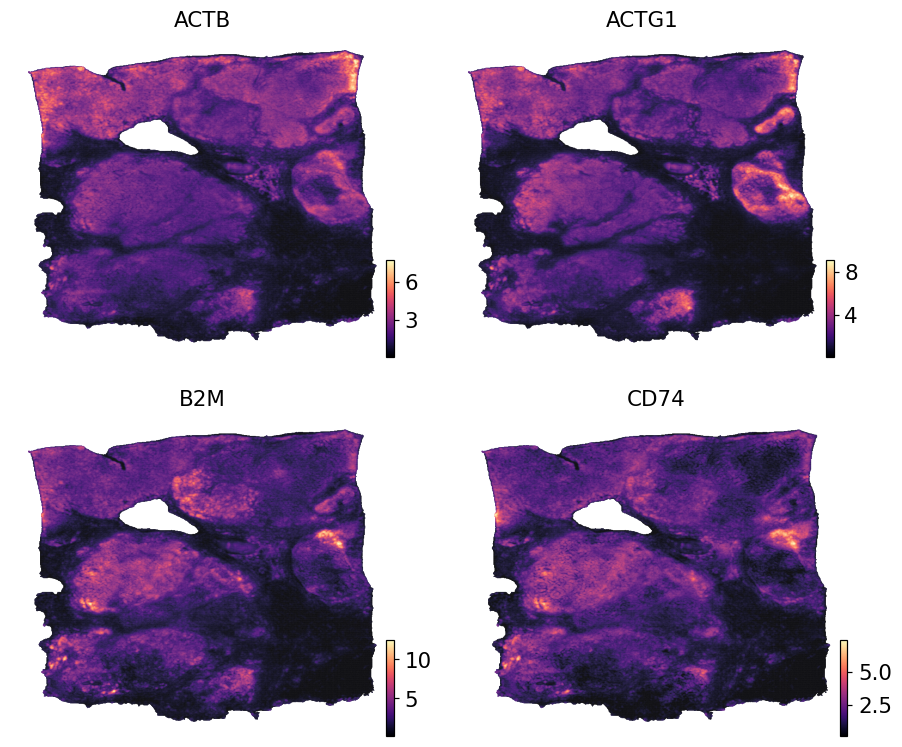
Visualise sub-spot expression#
Because pred carries pixel coordinates in obsm['spatial'], any spatial plotter (ov.pl.embedding, ov.pl.spatial, zs.pl.tiles) renders it without extra bookkeeping. The small dot size (s=1) is appropriate because the grid is very dense.
ov.pl.embedding(pred, basis='spatial',
                color=list(pred.var_names[:4]),
                cmap='magma', s=1, ncols=2, frameon=False)
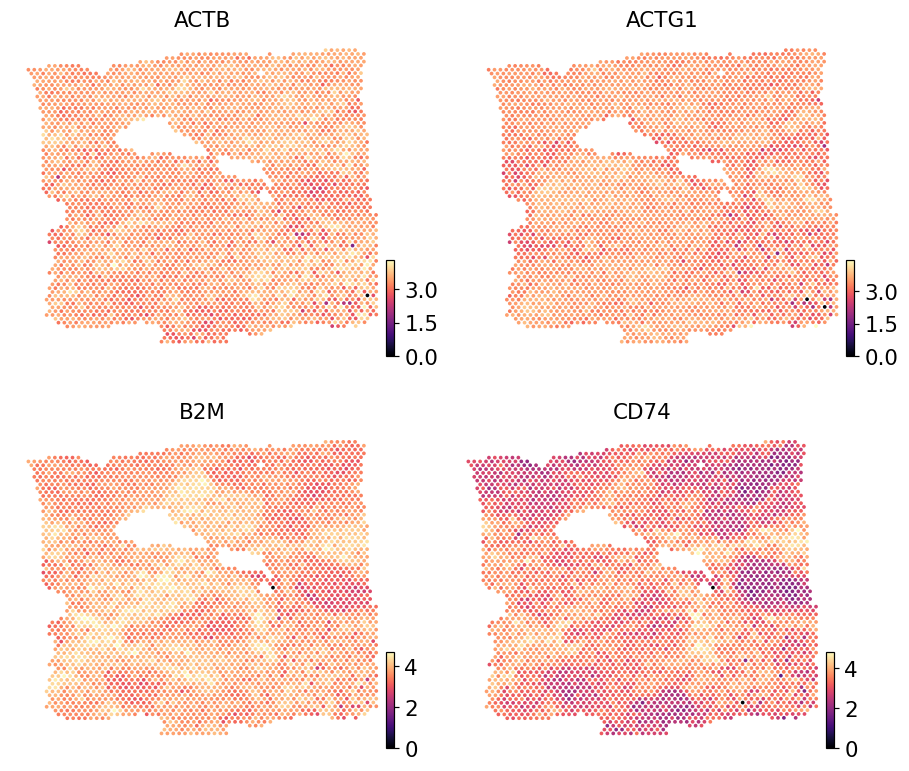
Real Visium counts for the same genes#
Render the same four imputed genes from the paired Visium reference so the sub-spot imputation can be eyeballed against the spot-level ground truth. The reference is log1p-normalised to match iStar’s output scale.
ref = adata.copy()
ov.pp.normalize_total(ref, target_sum=1e4)
ov.pp.log1p(ref)
ov.pl.embedding(ref, basis='spatial',
                color=list(pred.var_names[:4]),
                cmap='magma', s=24, ncols=2, frameon=False)
🔍 Count Normalization:
   Target sum: 10000.0
   Exclude highly expressed: False

✅ Count Normalization Completed Successfully!
   ✓ Processed: 3,798 cells × 36,601 genes
   ✓ Runtime: 0.05s
Where to go next#
The output AnnData feeds the rest of ov.space directly:
# spatial domain detection on the sub-spot grid
ov.space.pySTAGATE(pred, n_domains=8, radius=20)

# spatially-variable genes
pred = ov.space.svg(pred, mode='prost', n_svgs=200)

# marker enrichment for cell-type calling
ov.single.cosg(pred, groupby='STAGATE_domain')
For a head-to-head comparison with the spot-level backends on the same H&E, see the sibling tutorials (STPath, STFlow, HEST-FM).