Removing ambient / contamination RNA from droplet scRNA-seq#
Every droplet-based single-cell library is contaminated with ambient RNA — cell-free transcripts that leak out of stressed or lysed cells into the suspension and get co-encapsulated with real cells. This “soup” is captured and sequenced alongside each cell’s native transcriptome, so every cell barcode carries a background of transcripts it never expressed.
Left uncorrected, ambient RNA is not harmless noise:
it inflates marker genes in cell types that never expressed them — a T-cell barcode picks up haemoglobin from lysed erythrocytes, a neuron picks up a glial marker;
it distorts differential expression and cluster annotation, and produces phantom “doublet-like” or “low-quality” populations;
it scales with the soup concentration, so it is worst exactly in the samples that are hardest to dissociate (tumours, brain, frozen tissue).
Several methods estimate and subtract this background:
SoupX (Young & Behjati, GigaScience 2020) — reads the soup profile out of the empty droplets and subtracts a per-cell fraction.
DecontX (Yang et al., Genome Biology 2020) — a variational-EM model that needs a clustered matrix, no empty droplets required.
FastCAR (Berg et al. 2023) — deterministic per-gene subtraction from the empty-droplet ambient profile.
scCDC (Wang et al. 2024) — corrects only the Global-Contamination-causing Genes, deliberately conservative.
CellBender (Fleming et al., Nature Methods 2023) — a deep generative model; best overall in benchmarks but GPU-heavy.
ov.pp.ambient threads the four native, pip-installable backends
(pysoupx, pydecontx, pyfastcar, pysccdc) behind a single
remove_ambient dispatcher, and adds diagnostics that audit the
correction.
Where this step belongs. Ambient removal operates on raw counts, so it runs after cell calling (you need the filtered cells, and for SoupX / FastCAR also the empty droplets) and before normalization, HVG selection and clustering. In this tutorial we cluster first only because DecontX / scCDC need cluster labels — in a real pipeline you would do a quick preliminary clustering, decontaminate, then re-run the full downstream analysis on the cleaned counts.
1. Load a real raw 10x dataset#
ov.datasets.pbmc_raw_10x() downloads the 10x Genomics pbmc_1k_v3
dataset (peripheral-blood mononuclear cells, Chromium 3’ v3, processed
with Cell Ranger 3.0.0). With raw_droplets=True it returns two
AnnData objects:
cells— the filtered real cells (1,222 cells x 15,300 genes, raw UMI counts in.X);raw— the raw unfiltered droplet matrix (13,222 droplets = the 1,222 cells plus 12,000 empty droplets).
SoupX and FastCAR build their soup profile from those empty droplets, so
they need the raw object; DecontX and scCDC work from the filtered,
clustered cells alone.
import omicverse as ov
import scanpy as sc
import numpy as np
import matplotlib.pyplot as plt

ov.plot_set()
🔬 Starting plot initialization...
🧬 Detecting GPU devices…
🚫 No GPU devices found (CUDA/MPS/ROCm/XPU)

   ____            _     _    __
  / __ \____ ___  (_)___| |  / /__  _____________
 / / / / __ `__ \/ / ___/ | / / _ \/ ___/ ___/ _ \
/ /_/ / / / / / / / /__ | |/ /  __/ /  (__  )  __/
\____/_/ /_/ /_/_/\___/ |___/\___/_/  /____/\___/

🔖 Version: 2.2.1rc1   📚 Tutorials: https://omicverse.readthedocs.io/
✅ plot_set complete.
cells, raw = ov.datasets.pbmc_raw_10x(raw_droplets=True)
cells, raw
🔍 Downloading data to ./data/pbmc_raw_10x_cells.h5ad
⚠️ File ./data/pbmc_raw_10x_cells.h5ad already exists
🔍 Downloading data to ./data/pbmc_raw_10x_raw.h5ad
⚠️ File ./data/pbmc_raw_10x_raw.h5ad already exists
(AnnData object with n_obs × n_vars = 1222 × 15300
     obs: 'n_counts', 'n_genes'
     var: 'gene_ids', 'feature_types', 'genome'
     uns: 'dataset',
 AnnData object with n_obs × n_vars = 13222 × 15300
     obs: 'droplet_type', 'n_counts'
     var: 'gene_ids', 'feature_types', 'genome'
     uns: 'dataset')
# the raw matrix mixes real cells and empty droplets
raw.obs['droplet_type'].value_counts()
droplet_type
empty    12000
cell      1222
Name: count, dtype: int64
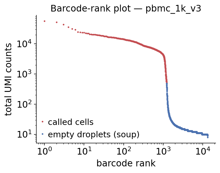
The barcode-rank plot#
The classic way to see the soup is the barcode-rank plot: total UMIs per droplet, sorted from highest to lowest on a log-log scale. Real cells sit on the high plateau; the long low tail is empty droplets that contain only ambient RNA — that tail is the soup profile SoupX and FastCAR estimate from.
counts = np.asarray(raw.X.sum(axis=1)).ravel()
order = np.argsort(counts)[::-1]
is_cell = (raw.obs['droplet_type'] == 'cell').to_numpy()[order]

fig, ax = plt.subplots(figsize=(5, 4))
rank = np.arange(1, len(counts) + 1)
ax.loglog(rank[is_cell], counts[order][is_cell], '.', ms=3,
          color='#C44E52', label='called cells')
ax.loglog(rank[~is_cell], counts[order][~is_cell], '.', ms=3,
          color='#4C72B0', label='empty droplets (soup)')
ax.set_xlabel('barcode rank')
ax.set_ylabel('total UMI counts')
ax.set_title('Barcode-rank plot — pbmc_1k_v3')
ax.legend(frameon=False)
ax.spines[['top', 'right']].set_visible(False)
plt.tight_layout()
plt.show()
2. A quick clustering#
DecontX and scCDC need cluster labels, and SoupX uses them to
auto-estimate the contamination fraction. We run a standard omicverse
preprocessing + Leiden pipeline on a working copy, then transfer the
labels and the UMAP back onto the raw-count cells object — ambient
removal must operate on raw counts across all genes, not on the
log-normalised HVG subset.
work = cells.copy()
work = ov.pp.preprocess(work, mode='shiftlog|pearson', n_HVGs=2000)
work.raw = work
work = work[:, work.var.highly_variable_features].copy()
🔍 [2026-05-22 00:17:46] Running preprocessing in 'cpu' mode...
Begin robust gene identification
    After filtration, 15300/15300 genes are kept.
    Among 15300 genes, 15300 genes are robust.
✅ Robust gene identification completed successfully.
Begin size normalization: shiftlog and HVGs selection pearson

🔍 Count Normalization:
   Target sum: 500000.0
   Exclude highly expressed: True
   Max fraction threshold: 0.2
   ⚠️ Excluding 5 highly-expressed genes from normalization computation
   Excluded genes: ['IGKC', 'HBB', 'MALAT1', 'MT-CO1', 'MT-CO3']

✅ Count Normalization Completed Successfully!
   ✓ Processed: 1,222 cells × 15,300 genes
   ✓ Runtime: 0.07s

🔍 Highly Variable Genes Selection (Experimental):
   Method: pearson_residuals
   Target genes: 2,000
   Theta (overdispersion): 100
✅ Experimental HVG Selection Completed Successfully!
   ✓ Selected: 2,000 highly variable genes out of 15,300 total (13.1%)
   ✓ Results added to AnnData object:
     • 'highly_variable': Boolean vector (adata.var)
     • 'highly_variable_rank': Float vector (adata.var)
     • 'highly_variable_nbatches': Int vector (adata.var)
     • 'highly_variable_intersection': Boolean vector (adata.var)
     • 'means': Float vector (adata.var)
     • 'variances': Float vector (adata.var)
     • 'residual_variances': Float vector (adata.var)
    Time to analyze data in cpu: 1.31 seconds.
✅ Preprocessing completed successfully.
    Added:
        'highly_variable_features', boolean vector (adata.var)
        'means', float vector (adata.var)
        'variances', float vector (adata.var)
        'residual_variances', float vector (adata.var)
        'counts', raw counts layer (adata.layers)
    End of size normalization: shiftlog and HVGs selection pearson

╭─ SUMMARY: preprocess ──────────────────────────────────────────────╮
│  Duration: 1.3926s                                                 │
│  Shape:    1,222 x 15,300 (Unchanged)                              │
│                                                                    │
│  CHANGES DETECTED                                                  │
│  ────────────────                                                  │
│  ● VAR    │ ✚ highly_variable (bool)                               │
│           │ ✚ highly_variable_features (bool)                      │
│           │ ✚ highly_variable_rank (float)                         │
│           │ ✚ means (float)                                        │
│           │ ✚ n_cells (int)                                        │
│           │ ✚ percent_cells (float)                                │
│           │ ✚ residual_variances (float)                           │
│           │ ✚ robust (bool)                                        │
│           │ ✚ variances (float)                                    │
│                                                                    │
│  ● UNS    │ ✚ REFERENCE_MANU                                       │
│           │ ✚ _ov_provenance                                       │
│           │ ✚ history_log                                          │
│           │ ✚ hvg                                                  │
│           │ ✚ log1p                                                │
│           │ ✚ status                                               │
│           │ ✚ status_args                                          │
│                                                                    │
│  ● LAYERS │ ✚ counts (sparse matrix, 1222x15300)                   │
│                                                                    │
╰────────────────────────────────────────────────────────────────────╯
ov.pp.scale(work)
ov.pp.pca(work, layer='scaled', n_pcs=30)
ov.pp.neighbors(work, n_neighbors=15, n_pcs=30, use_rep='scaled|original|X_pca')
ov.pp.leiden(work, resolution=1.0)
ov.pp.umap(work)
╭─ SUMMARY: scale ───────────────────────────────────────────────────╮
│  Duration: 0.0259s                                                 │
│  Shape:    1,222 x 2,000 (Unchanged)                               │
│                                                                    │
│  CHANGES DETECTED                                                  │
│  ────────────────                                                  │
│  ● LAYERS │ ✚ scaled (array, 1222x2000)                            │
│                                                                    │
╰────────────────────────────────────────────────────────────────────╯
computing PCA🔍
    with n_comps=30
   🖥️ Using sklearn PCA for CPU computation
   🖥️ sklearn PCA backend: CPU computation
   📊 PCA input data type: ArrayView, shape: (1222, 2000), dtype: float64
🔧 PCA solver used: covariance_eigh
    finished✅ (5.87s)

╭─ SUMMARY: pca ─────────────────────────────────────────────────────╮
│  Duration: 5.8701s                                                 │
│  Shape:    1,222 x 2,000 (Unchanged)                               │
│                                                                    │
│  CHANGES DETECTED                                                  │
│  ────────────────                                                  │
│  ● UNS    │ ✚ pca                                                  │
│           │ └─ params: {'zero_center': True, 'use_highly_variable': Tr...│
│           │ ✚ scaled|original|cum_sum_eigenvalues                  │
│           │ ✚ scaled|original|pca_var_ratios                       │
│                                                                    │
│  ● OBSM   │ ✚ X_pca (array, 1222x30)                               │
│           │ ✚ scaled|original|X_pca (array, 1222x30)               │
│                                                                    │
╰────────────────────────────────────────────────────────────────────╯
🖥️ Using Scanpy CPU to calculate neighbors...

🔍 K-Nearest Neighbors Graph Construction:
   Mode: cpu
   Neighbors: 15
   Method: umap
   Metric: euclidean
   Representation: scaled|original|X_pca
   PCs used: 30
   🔍 Computing neighbor distances...
🔍 Computing connectivity matrix...
   💡 Using UMAP-style connectivity
✓ Graph is fully connected

✅ KNN Graph Construction Completed Successfully!
   ✓ Processed: 1,222 cells with 15 neighbors each
   ✓ Results added to AnnData object:
     • 'neighbors': Neighbors metadata (adata.uns)
     • 'distances': Distance matrix (adata.obsp)
     • 'connectivities': Connectivity matrix (adata.obsp)

╭─ SUMMARY: neighbors ───────────────────────────────────────────────╮
│  Duration: 11.3594s                                                │
│  Shape:    1,222 x 2,000 (Unchanged)                               │
│                                                                    │
│  CHANGES DETECTED                                                  │
│  ────────────────                                                  │
│  ● UNS    │ ✚ neighbors                                            │
│           │ └─ params: {'n_neighbors': 15, 'method': 'umap', 'random_s...│
│                                                                    │
│  ● OBSP   │ ✚ connectivities (sparse matrix, 1222x1222)            │
│           │ ✚ distances (sparse matrix, 1222x1222)                 │
│                                                                    │
╰────────────────────────────────────────────────────────────────────╯
🖥️ Using Scanpy CPU Leiden...
running Leiden clustering
    finished (0.06s)
    found 13 clusters and added
    'leiden', the cluster labels (adata.obs, categorical)

╭─ SUMMARY: leiden ──────────────────────────────────────────────────╮
│  Duration: 0.0586s                                                 │
│  Shape:    1,222 x 2,000 (Unchanged)                               │
│                                                                    │
│  CHANGES DETECTED                                                  │
│  ────────────────                                                  │
│  ● OBS    │ ✚ leiden (category)                                    │
│                                                                    │
│  ● UNS    │ ✚ leiden                                               │
│           │ └─ params: {'resolution': 1.0, 'random_state': 0, 'n_itera...│
│                                                                    │
╰────────────────────────────────────────────────────────────────────╯
🔍 [2026-05-22 00:18:04] Running UMAP in 'cpu' mode...
🖥️ Using Scanpy CPU UMAP...

🔍 UMAP Dimensionality Reduction:
   Mode: cpu
   Method: umap
   Components: 2
   Min distance: 0.5
{'n_neighbors': 15, 'method': 'umap', 'random_state': 0, 'metric': 'euclidean', 'use_rep': 'scaled|original|X_pca', 'n_pcs': 30}
   🔍 Computing UMAP parameters...
   🔍 Computing UMAP embedding (classic method)...
✅ UMAP Dimensionality Reduction Completed Successfully!
   ✓ Embedding shape: 1,222 cells × 2 dimensions
   ✓ Results added to AnnData object:
     • 'X_umap': UMAP coordinates (adata.obsm)
     • 'umap': UMAP parameters (adata.uns)
✅ UMAP completed successfully.

╭─ SUMMARY: umap ────────────────────────────────────────────────────╮
│  Duration: 0.794s                                                  │
│  Shape:    1,222 x 2,000 (Unchanged)                               │
│                                                                    │
│  CHANGES DETECTED                                                  │
│  ────────────────                                                  │
│  ● UNS    │ ✚ umap                                                 │
│           │ └─ params: {'a': np.float64(0.5830300203414425), 'b': np.f...│
│                                                                    │
│  ● OBSM   │ ✚ X_umap (array, 1222x2)                               │
│                                                                    │
╰────────────────────────────────────────────────────────────────────╯
# transfer the cluster labels + embedding onto the raw-count AnnData
cells.obs['leiden'] = work.obs['leiden'].values
cells.obsm['X_umap'] = work.obsm['X_umap']
cells.obs['leiden'].value_counts()
leiden
0     224
1     182
2     125
3     122
4     108
5      72
6      69
7      64
8      63
9      57
10     54
11     47
12     35
Name: count, dtype: int64
3. Run remove_ambient with each native method#
ov.pp.ambient.remove_ambient is a single method= dispatcher. It
writes the decontaminated counts back into .X, keeps the original
counts in layers['ambient_raw'], stores the per-cell contamination
fraction in obs['ambient_contamination'], and records method metadata
in uns['ambient'].
SoupX / FastCAR need the raw unfiltered matrix — pass
raw=.DecontX / scCDC need cluster labels — pass
cluster_key=.
We run all four on independent copies so we can compare them.
ad_soupx = cells.copy()
ov.pp.ambient.remove_ambient(ad_soupx, method='soupx', raw=raw,
                             cluster_key='leiden', verbose=True)
773 genes passed tf-idf cut-off and 103 soup quantile filter. Taking the top 100.
Using 952 independent estimates of rho.
Estimated global rho of 0.01
[ov.pp.ambient] method=soupx  mean contamination=0.0100  genes corrected=15300
AnnData object with n_obs × n_vars = 1222 × 15300
    obs: 'n_counts', 'n_genes', 'leiden', 'ambient_contamination'
    var: 'gene_ids', 'feature_types', 'genome'
    uns: 'dataset', 'ambient'
    obsm: 'X_umap'
    layers: 'ambient_raw'
ad_decontx = cells.copy()
ov.pp.ambient.remove_ambient(ad_decontx, method='decontx',
                             cluster_key='leiden', verbose=True)
DecontX: analysing batch 'all_cells' (1222 cells)
iter 10 | converge: 0.03146
iter 20 | converge: 0.0201
iter 30 | converge: 0.009111
iter 40 | converge: 0.004174
iter 50 | converge: 0.002953
iter 60 | converge: 0.002275
iter 70 | converge: 0.001807
iter 80 | converge: 0.002192
iter 90 | converge: 0.00159
iter 100 | converge: 0.001244
iter 110 | converge: 0.001005
  iter 111 | converge: 0.001
[ov.pp.ambient] method=decontx  mean contamination=0.0856  genes corrected=15300
AnnData object with n_obs × n_vars = 1222 × 15300
    obs: 'n_counts', 'n_genes', 'leiden', 'ambient_contamination'
    var: 'gene_ids', 'feature_types', 'genome'
    uns: 'dataset', 'ambient'
    obsm: 'X_umap'
    layers: 'ambient_raw'
ad_fastcar = cells.copy()
ov.pp.ambient.remove_ambient(ad_fastcar, method='fastcar', raw=raw,
                             verbose=True)
[ov.pp.ambient] method=fastcar mean contamination=0.0941 genes corrected=247
AnnData object with n_obs × n_vars = 1222 × 15300
    obs: 'n_counts', 'n_genes', 'leiden', 'ambient_contamination'
    var: 'gene_ids', 'feature_types', 'genome'
    uns: 'dataset', 'ambient'
    obsm: 'X_umap'
    layers: 'ambient_raw'
ad_sccdc = cells.copy()
ov.pp.ambient.remove_ambient(ad_sccdc, method='sccdc',
                             cluster_key='leiden', verbose=True)
[ov.pp.ambient] method=sccdc mean contamination=0.1317 genes corrected=59
AnnData object with n_obs × n_vars = 1222 × 15300
    obs: 'n_counts', 'n_genes', 'leiden', 'ambient_contamination'
    var: 'gene_ids', 'feature_types', 'genome'
    uns: 'dataset', 'ambient'
    obsm: 'X_umap'
    layers: 'ambient_raw'
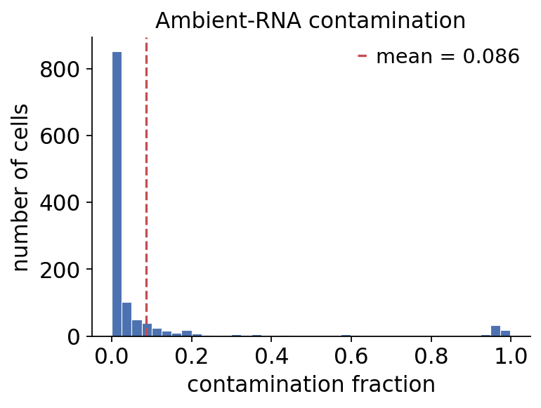
Per-cell contamination fraction#
Each run populates obs['ambient_contamination']. The four methods make
different modelling assumptions, so they will not agree on a single
number — that disagreement is itself informative, and the diagnostics
below let us judge the corrections rather than trust them blindly.
import pandas as pd
summary = pd.DataFrame({
    'soupx':   [ad_soupx.uns['ambient']['contamination_fraction']],
    'decontx': [ad_decontx.uns['ambient']['contamination_fraction']],
    'fastcar': [ad_fastcar.uns['ambient']['contamination_fraction']],
    'sccdc':   [ad_sccdc.uns['ambient']['contamination_fraction']],
}, index=['mean contamination fraction'])
summary.T
| mean contamination fraction | |
|---|---|
| soupx | 0.010000 |
| decontx | 0.085641 |
| fastcar | 0.094148 |
| sccdc | 0.131743 |
# distribution of the per-cell contamination fraction (DecontX run)
ov.pp.ambient.plot_contamination(ad_decontx)
plt.show()
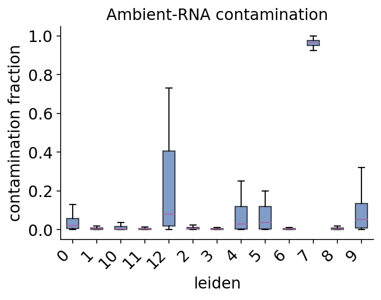
# contamination tends to track cell type — show it per Leiden cluster
ov.pp.ambient.plot_contamination(ad_decontx, groupby='leiden')
plt.show()
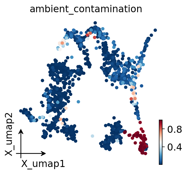
# overlay the contamination fraction on the UMAP
ov.pl.embedding(ad_decontx, basis='X_umap', color='ambient_contamination',
                frameon='small', show=False)
plt.show()
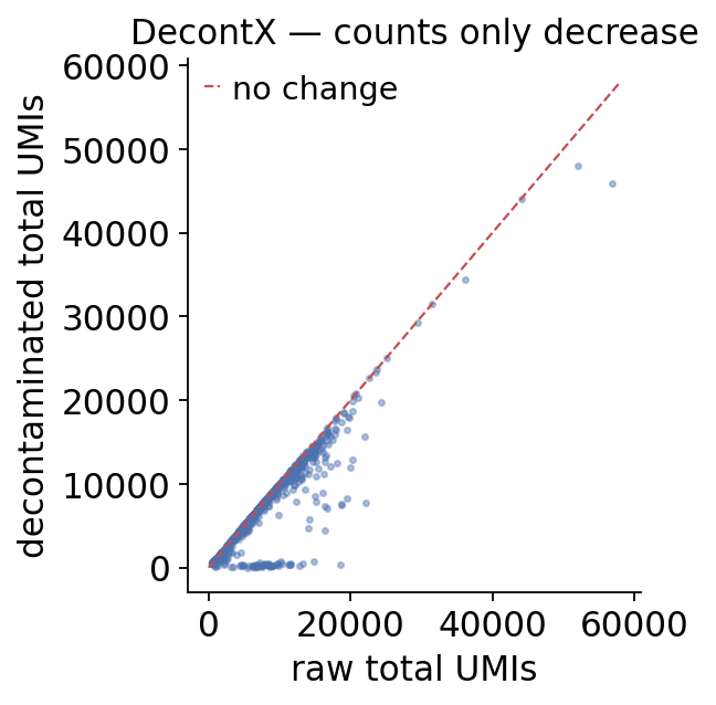
Corrected vs raw counts#
The decontaminated counts are now in .X; the originals are preserved
in layers['ambient_raw']. The total UMIs only ever go down —
ambient removal subtracts, it never adds.
raw_tot = np.asarray(ad_decontx.layers['ambient_raw'].sum(axis=1)).ravel()
cor_tot = np.asarray(ad_decontx.X.sum(axis=1)).ravel()

fig, ax = plt.subplots(figsize=(4.2, 4.2))
ax.scatter(raw_tot, cor_tot, s=5, alpha=0.4, color='#4C72B0')
lim = [0, raw_tot.max() * 1.02]
ax.plot(lim, lim, '--', color='#C44E52', lw=1, label='no change')
ax.set_xlabel('raw total UMIs')
ax.set_ylabel('decontaminated total UMIs')
ax.set_title('DecontX — counts only decrease')
ax.legend(frameon=False)
ax.spines[['top', 'right']].set_visible(False)
plt.tight_layout()
plt.show()
4. Diagnostics#
ov.pp.ambient ships read-only audits that check whether a correction
behaved sensibly — they do not modify the data.
4.1 Negative-marker check#
A correct decontamination should drive a cell-type-specific marker
back toward zero in the cell types that biologically do not express
it. Haemoglobin HBB is the textbook example: it is hugely expressed
in erythrocytes/platelet contamination and leaks into every other
barcode as soup. ambient_negative_marker_check compares the raw vs
corrected mean of HBB across cell types and reports the fold reduction
in the cell types that should be HBB-negative.
hbb = ov.pp.ambient.ambient_negative_marker_check(
    ad_decontx, 'HBB', 'leiden')
hbb[['n_cells', 'raw_mean', 'corrected_mean', 'fold_reduction']].round(3)
| n_cells | raw_mean | corrected_mean | fold_reduction | |
|---|---|---|---|---|
| celltype | ||||
| 0 | 224 | 0.000 | 0.000 | inf |
| 2 | 125 | 0.000 | 0.000 | inf |
| 8 | 63 | 0.000 | 0.000 | inf |
| 1 | 182 | 0.049 | 0.047 | 1.057000e+00 |
| 7 | 64 | 0.016 | 0.000 | 7.470206e+16 |
| 11 | 47 | 0.000 | 0.000 | inf |
| 6 | 69 | 0.000 | 0.000 | inf |
| 9 | 57 | 0.000 | 0.000 | inf |
| 4 | 108 | 4.056 | 4.056 | 1.000000e+00 |
| 10 | 54 | 0.000 | 0.000 | inf |
| 5 | 72 | 0.000 | 0.000 | inf |
| 3 | 122 | 0.000 | 0.000 | inf |
| 12 | 35 | 0.000 | 0.000 | inf |
# the aggregate over the HBB-negative cell types
hbb.attrs['summary']
{'marker': 'HBB',
 'positive_celltypes': ['4'],
 'n_negative_celltypes': 12,
 'neg_raw_mean': 0.0054229625190297765,
 'neg_corrected_mean': 0.0038977974782859297,
 'neg_fold_reduction': 1.3912889392638592}
The positive cell type (highest raw HBB — the erythroid/platelet cluster) keeps its HBB, while the HBB-negative cell types see their residual haemoglobin signal pushed down. That is exactly the behaviour ambient removal should produce: soup stripped, biology preserved.
4.2 Count-integrity check#
A trustworthy correction only subtracts: no matrix entry may grow,
and only the contaminated genes should change at all.
count_integrity_check verifies this against the 2026 ambient-RNA
benchmark count-integrity criterion.
integ = ov.pp.ambient.count_integrity_check(
    ad_decontx.layers['ambient_raw'], ad_decontx.X)
integ
{'passed': True,
 'n_entries': 18696600,
 'n_increased': 0,
 'max_increase': 0.0,
 'n_unchanged': 16203657,
 'frac_unchanged': 0.8666632970700555,
 'frac_changed': 0.13333670292994448,
 'total_raw': 9230791.0,
 'total_corrected': 8344633.546892991,
 'total_removed': 886157.4531070087,
 'removed_fraction': 0.09600016435287168}
4.3 Contamination report#
contamination_report reads the metadata remove_ambient wrote into
obs / uns and returns a compact one-row summary per method.
report = pd.concat([
    ov.pp.ambient.contamination_report(ad_soupx),
    ov.pp.ambient.contamination_report(ad_decontx),
    ov.pp.ambient.contamination_report(ad_fastcar),
    ov.pp.ambient.contamination_report(ad_sccdc),
], ignore_index=True)
report
| method | n_cells | n_genes | genes_corrected | mean_contamination | median_contamination | min_contamination | max_contamination | integrity_passed | removed_fraction | frac_genes_changed | |
|---|---|---|---|---|---|---|---|---|---|---|---|
| 0 | soupx | 1222 | 15300 | 15300 | 0.010000 | 0.010000 | 0.010000 | 0.010000 | True | 0.010000 | 0.126952 |
| 1 | decontx | 1222 | 15300 | 15300 | 0.085641 | 0.007672 | 0.000039 | 0.998265 | True | 0.096000 | 0.133337 |
| 2 | fastcar | 1222 | 15300 | 247 | 0.094148 | 0.083521 | 0.009843 | 0.382253 | True | 0.070733 | 0.013277 |
| 3 | sccdc | 1222 | 15300 | 59 | 0.131743 | 0.103346 | 0.001969 | 0.802548 | True | 0.094104 | 0.003494 |
5. Ground-truth validation on a species-mixing dataset#
On real PBMCs we have no ground truth for the soup — we can only check that the correction behaves sensibly. The human-mouse species-mixing (“barnyard”) experiment removes that ambiguity.
ov.datasets.hgmm_mixture() loads the 10x hgmm_1k_v3 dataset: a
1:1 mix of human (HEK293T) and mouse (NIH3T3) cells, sequenced against a
combined hg19 + mm10 reference. Because the two species share no
genes, any transcript mapped to the other species inside a cell is
unambiguous ambient contamination. The per-cell minor-species read
fraction is therefore a direct, label-free measure of soup — and a real
correction must reduce it.
hg_cells, hg_raw = ov.datasets.hgmm_mixture(raw_droplets=True)
hg_cells.obs['species'].value_counts()
🔍 Downloading data to ./data/hgmm_mixture_cells.h5ad
⚠️ File ./data/hgmm_mixture_cells.h5ad already exists
🔍 Downloading data to ./data/hgmm_mixture_raw.h5ad
⚠️ File ./data/hgmm_mixture_raw.h5ad already exists
species
mouse    544
human    495
mixed      7
Name: count, dtype: int64
We split the genes by genome (hg19 vs mm10) and define the
cross-species fraction of a count matrix as the minor-species share
of each cell’s reads — min(human_frac, mouse_frac). With the genome
masks fixed, this is a short vectorised expression we reuse for the raw
matrix and for each decontaminated matrix.
# genome masks — fixed once, the soup measurement reuses them
genome = hg_cells.var['genome'].to_numpy()
hg_mask = genome == 'hg19'
mm_mask = genome == 'mm10'
print(f'{hg_mask.sum()} human (hg19) genes, {mm_mask.sum()} mouse (mm10) genes')
16122 human (hg19) genes, 13862 mouse (mm10) genes
# ground-truth contamination of the RAW counts: minor-species read fraction
hg_umi = np.asarray(hg_cells.X[:, hg_mask].sum(axis=1)).ravel()
mm_umi = np.asarray(hg_cells.X[:, mm_mask].sum(axis=1)).ravel()
hg_frac = hg_umi / np.maximum(hg_umi + mm_umi, 1)
gt_raw = np.minimum(hg_frac, 1.0 - hg_frac)
print(f'ground-truth mean cross-species fraction: {gt_raw.mean():.4f}')
print(f'                            median:       {np.median(gt_raw):.4f}')
ground-truth mean cross-species fraction: 0.0075
                            median:       0.0045
Roughly 0.75 % of every cell’s reads come from the wrong species — that is the ambient contamination, measured without any model. Now we cluster the cells (the two species form cleanly separated clusters), run each backend, and recompute the cross-species fraction from the decontaminated counts.
hg_work = hg_cells.copy()
hg_work = ov.pp.preprocess(hg_work, mode='shiftlog|pearson', n_HVGs=2000)
hg_work.raw = hg_work
hg_work = hg_work[:, hg_work.var.highly_variable_features].copy()
ov.pp.scale(hg_work)
ov.pp.pca(hg_work, layer='scaled', n_pcs=30)
ov.pp.neighbors(hg_work, n_neighbors=15, n_pcs=30,
                use_rep='scaled|original|X_pca')
ov.pp.leiden(hg_work, resolution=0.5)
hg_cells.obs['leiden'] = hg_work.obs['leiden'].values
🔍 [2026-05-22 00:18:46] Running preprocessing in 'cpu' mode...
Begin robust gene identification
    After filtration, 29984/29984 genes are kept.
    Among 29984 genes, 29984 genes are robust.
✅ Robust gene identification completed successfully.
Begin size normalization: shiftlog and HVGs selection pearson
🔍 Count Normalization:
   Target sum: 500000.0
   Exclude highly expressed: True
   Max fraction threshold: 0.2
⚠️ Excluding 4 highly-expressed genes from normalization computation
   Excluded genes: ['hg19_MT-CO2', 'mm10_mt-Nd2', 'mm10_mt-Nd4', 'mm10_mt-Cytb']

✅ Count Normalization Completed Successfully!
   ✓ Processed: 1,046 cells × 29,984 genes
   ✓ Runtime: 0.11s

🔍 Highly Variable Genes Selection (Experimental):
   Method: pearson_residuals
   Target genes: 2,000
   Theta (overdispersion): 100
✅ Experimental HVG Selection Completed Successfully!
   ✓ Selected: 2,000 highly variable genes out of 29,984 total (6.7%)
   ✓ Results added to AnnData object:
     • 'highly_variable': Boolean vector (adata.var)
     • 'highly_variable_rank': Float vector (adata.var)
     • 'highly_variable_nbatches': Int vector (adata.var)
     • 'highly_variable_intersection': Boolean vector (adata.var)
     • 'means': Float vector (adata.var)
     • 'variances': Float vector (adata.var)
     • 'residual_variances': Float vector (adata.var)
    Time to analyze data in cpu: 0.97 seconds.
✅ Preprocessing completed successfully.
    Added:
        'highly_variable_features', boolean vector (adata.var)
        'means', float vector (adata.var)
        'variances', float vector (adata.var)
        'residual_variances', float vector (adata.var)
        'counts', raw counts layer (adata.layers)
    End of size normalization: shiftlog and HVGs selection pearson

╭─ SUMMARY: preprocess ──────────────────────────────────────────────╮
│  Duration: 1.1255s                                                 │
│  Shape:    1,046 x 29,984 (Unchanged)                              │
│                                                                    │
│  CHANGES DETECTED                                                  │
│  ────────────────                                                  │
│  ● VAR    │ ✚ highly_variable (bool)                               │
│           │ ✚ highly_variable_features (bool)                      │
│           │ ✚ highly_variable_rank (float)                         │
│           │ ✚ means (float)                                        │
│           │ ✚ n_cells (int)                                        │
│           │ ✚ percent_cells (float)                                │
│           │ ✚ residual_variances (float)                           │
│           │ ✚ robust (bool)                                        │
│           │ ✚ variances (float)                                    │
│                                                                    │
│  ● UNS    │ ✚ REFERENCE_MANU                                       │
│           │ ✚ _ov_provenance                                       │
│           │ ✚ history_log                                          │
│           │ ✚ hvg                                                  │
│           │ ✚ log1p                                                │
│           │ ✚ status                                               │
│           │ ✚ status_args                                          │
│                                                                    │
│  ● LAYERS │ ✚ counts (sparse matrix, 1046x29984)                   │
│                                                                    │
╰────────────────────────────────────────────────────────────────────╯

╭─ SUMMARY: scale ───────────────────────────────────────────────────╮
│  Duration: 0.0273s                                                 │
│  Shape:    1,046 x 2,000 (Unchanged)                               │
│                                                                    │
│  CHANGES DETECTED                                                  │
│  ────────────────                                                  │
│  ● LAYERS │ ✚ scaled (array, 1046x2000)                            │
│                                                                    │
╰────────────────────────────────────────────────────────────────────╯
computing PCA🔍
    with n_comps=30
   🖥️ Using sklearn PCA for CPU computation
   🖥️ sklearn PCA backend: CPU computation
   📊 PCA input data type: ArrayView, shape: (1046, 2000), dtype: float64
🔧 PCA solver used: covariance_eigh
    finished✅ (1.94s)

╭─ SUMMARY: pca ─────────────────────────────────────────────────────╮
│  Duration: 1.9419s                                                 │
│  Shape:    1,046 x 2,000 (Unchanged)                               │
│                                                                    │
│  CHANGES DETECTED                                                  │
│  ────────────────                                                  │
│  ● UNS    │ ✚ pca                                                  │
│           │ └─ params: {'zero_center': True, 'use_highly_variable': Tr...│
│           │ ✚ scaled|original|cum_sum_eigenvalues                  │
│           │ ✚ scaled|original|pca_var_ratios                       │
│                                                                    │
│  ● OBSM   │ ✚ X_pca (array, 1046x30)                               │
│           │ ✚ scaled|original|X_pca (array, 1046x30)               │
│                                                                    │
╰────────────────────────────────────────────────────────────────────╯
🖥️ Using Scanpy CPU to calculate neighbors...

🔍 K-Nearest Neighbors Graph Construction:
   Mode: cpu
   Neighbors: 15
   Method: umap
   Metric: euclidean
   Representation: scaled|original|X_pca
   PCs used: 30
   🔍 Computing neighbor distances...
   🔍 Computing connectivity matrix...
   💡 Using UMAP-style connectivity
✓ Graph is fully connected

✅ KNN Graph Construction Completed Successfully!
   ✓ Processed: 1,046 cells with 15 neighbors each
   ✓ Results added to AnnData object:
     • 'neighbors': Neighbors metadata (adata.uns)
     • 'distances': Distance matrix (adata.obsp)
     • 'connectivities': Connectivity matrix (adata.obsp)

╭─ SUMMARY: neighbors ───────────────────────────────────────────────╮
│  Duration: 0.2066s                                                 │
│  Shape:    1,046 x 2,000 (Unchanged)                               │
│                                                                    │
│  CHANGES DETECTED                                                  │
│  ────────────────                                                  │
│  ● UNS    │ ✚ neighbors                                            │
│           │ └─ params: {'n_neighbors': 15, 'method': 'umap', 'random_s...│
│                                                                    │
│  ● OBSP   │ ✚ connectivities (sparse matrix, 1046x1046)            │
│           │ ✚ distances (sparse matrix, 1046x1046)                 │
│                                                                    │
╰────────────────────────────────────────────────────────────────────╯
🖥️ Using Scanpy CPU Leiden...
running Leiden clustering
    finished (0.04s)
    found 6 clusters and added
    'leiden', the cluster labels (adata.obs, categorical)

╭─ SUMMARY: leiden ──────────────────────────────────────────────────╮
│  Duration: 0.0386s                                                 │
│  Shape:    1,046 x 2,000 (Unchanged)                               │
│                                                                    │
│  CHANGES DETECTED                                                  │
│  ────────────────                                                  │
│  ● OBS    │ ✚ leiden (category)                                    │
│                                                                    │
│  ● UNS    │ ✚ leiden                                               │
│           │ └─ params: {'resolution': 0.5, 'random_state': 0, 'n_itera...│
│                                                                    │
╰────────────────────────────────────────────────────────────────────╯
# decontaminate with each native method and measure the residual soup
gt = {'raw (no correction)': gt_raw.mean()}
for method in ['soupx', 'decontx', 'fastcar', 'sccdc']:
    a = hg_cells.copy()
    if method in ('soupx', 'fastcar'):
        ov.pp.ambient.remove_ambient(a, method=method, raw=hg_raw,
                                     cluster_key='leiden')
    else:
        ov.pp.ambient.remove_ambient(a, method=method,
                                     cluster_key='leiden')
    hg_c = np.asarray(a.X[:, hg_mask].sum(axis=1)).ravel()
    mm_c = np.asarray(a.X[:, mm_mask].sum(axis=1)).ravel()
    f = hg_c / np.maximum(hg_c + mm_c, 1)
    gt[method] = float(np.minimum(f, 1.0 - f).mean())

gt_df = pd.DataFrame({'mean cross-species fraction': gt})
gt_df['reduction vs raw'] = 1.0 - gt_df['mean cross-species fraction'] / gt['raw (no correction)']
gt_df.round(4)
| mean cross-species fraction | reduction vs raw | |
|---|---|---|
| raw (no correction) | 0.0075 | 0.0000 |
| soupx | 0.0042 | 0.4452 |
| decontx | 0.0047 | 0.3797 |
| fastcar | 0.0042 | 0.4346 |
| sccdc | 0.0074 | 0.0181 |
fig, ax = plt.subplots(figsize=(5.5, 4.2), constrained_layout=True)
colors = ["#7f7f7f", "#4C72B0", "#55A868", "#C44E52", "#8172B3"]
ax.bar(gt_df.index, gt_df["mean cross-species fraction"], color=colors)
ax.axhline(gt["raw (no correction)"], ls="--", lw=1, color="#7f7f7f")
ax.set_ylabel("mean cross-species read fraction")
ax.set_title("hgmm species-mixing — ground-truth contamination", fontsize=11)
for tick in ax.get_xticklabels():
    tick.set_rotation(30)
    tick.set_ha("right")
ax.spines[["top", "right"]].set_visible(False)
plt.show()
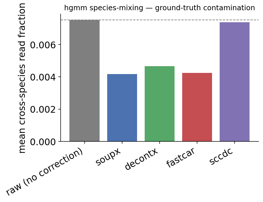
This is the real test: the cross-species read fraction is a quantity no method can see during fitting, yet every backend reduces it. The empty-droplet methods (SoupX, FastCAR) and the EM model (DecontX) all strip a substantial share of the wrong-species reads; scCDC, which by design only touches Global-Contamination-causing Genes, moves it least — the expected behaviour of a deliberately conservative method.
6. Choosing a method#
The four native backends — plus the deep-learning options — make different trade-offs. The research consensus, and the behaviour seen above:
Method |
Needs |
Strengths |
Watch out for |
|---|---|---|---|
SoupX |
raw matrix + empty droplets; clusters for auto-rho |
gentle, interpretable, fast; reads the soup directly from empty droplets |
conservative — under-corrects clean datasets |
DecontX |
filtered, clustered matrix |
no empty droplets required; per-cell variational estimate |
can over-correct if clustering is poor |
FastCAR |
raw matrix + empty droplets |
deterministic per-gene subtraction; very fast |
tuned by hard cutoffs ( |
scCDC |
filtered, clustered matrix |
anti-over-correction — only fixes contamination-causing genes |
corrects few genes; leaves most soup if it is diffuse |
CellBender |
raw 10x h5 (GPU) |
best overall in benchmarks; jointly calls cells + removes background |
heavyweight, GPU, run via its own CLI |
scAR |
raw matrix (GPU) |
deep ambient denoising |
heavyweight, GPU |
Practical guidance:
Have empty droplets and want a safe default — SoupX. It rarely hurts and is easy to reason about.
Only have a filtered matrix (a public h5ad, no raw droplets) — DecontX or scCDC.
Worried about over-correction of biologically real markers — scCDC.
Compute budget and a GPU — CellBender generally wins benchmarks, but is heavyweight;
ov.pp.ambientkeeps its wrapper thin and points you at CellBender’s ownremove-backgroundCLI, then load the result withov.read.
Whatever you pick, audit it: ambient_negative_marker_check,
count_integrity_check and — when you have one — a ground-truth signal
like the cross-species fraction. Then continue the normal workflow
(normalize, HVG, cluster, annotate) on the decontaminated .X.