B-cell receptor repertoire analysis with ov.airr#
When you are vaccinated, the immune response is written into the B-cell receptor (BCR) repertoire. Each naive B cell carries a unique immunoglobulin heavy chain (IgH), assembled by V(D)J recombination. On encountering antigen, responding B cells enter germinal centres and undergo affinity maturation — a Darwinian cycle of:
Clonal expansion — antigen-specific B cells proliferate, so their IgH sequences come to dominate the repertoire.
Somatic hypermutation (SHM) — the enzyme AID introduces point mutations into the rearranged V(D)J at a rate ~10^6-fold above background.
Selection — variants with higher antigen affinity are preferentially retained; the mutations that improve binding accumulate in the antigen-contacting CDRs, while the structural framework regions (FWRs) are kept intact by purifying selection.
Class switching — selected clones switch from IgM/IgD to IgG/IgA.
A BCR repertoire snapshot therefore carries a molecular fossil record of this process. This tutorial reconstructs that record.
The dataset#
We use the Laserson et al. 2014 influenza-vaccination IgH repertoire
(PNAS 2014, PMID 24639495) –
high-throughput IgH sequencing from one subject at two timepoints:
pre-vaccination (-1h) and day 7 post-vaccination (+7d), the peak
of the plasmablast response. The data are in standard AIRR rearrangement
format: one row per IgH sequence, with V/D/J gene calls, the CDR3 junction,
and IMGT-numbered alignments to the inferred germline.
What ov.airr provides#
ov.airr threads the Immcantation B-cell toolchain behind one registered
API – clonal clustering (pyscoper), somatic hypermutation and BASELINe
selection (pyshazam), Ig genotyping (pytigger) and B-cell phylogenetics
(pydowser). Functions take a plain AIRR-format pandas.DataFrame, so the
whole analysis stays tabular and inspectable.
0. Setup#
The B-cell side of ov.airr is table-native – there is no AnnData here, just
an AIRR DataFrame that each step annotates with new columns.
import omicverse as ov
import numpy as np
import pandas as pd
import matplotlib.pyplot as plt
ov.plot_set()
🔬 Starting plot initialization...
🧬 Detecting GPU devices…
🚫 No GPU devices found (CUDA/MPS/ROCm/XPU)

   ____            _     _    __
  / __ \____ ___  (_)___| |  / /__  _____________
 / / / / __ `__ \/ / ___/ | / / _ \/ ___/ ___/ _ \
/ /_/ / / / / / / / /__ | |/ /  __/ /  (__  )  __/
\____/_/ /_/ /_/_/\___/ |___/\___/_/  /____/\___/

🔖 Version: 2.2.1rc1   📚 Tutorials: https://omicverse.readthedocs.io/
✅ plot_set complete.
1. Load the IgH repertoire#
ov.datasets.airr_bcr() returns the Laserson 2014 IgH table as an
AIRR-format DataFrame. Each row is one rearranged heavy chain.
bcr = ov.datasets.airr_bcr()
print(f"sequences: {bcr.shape[0]}   columns: {bcr.shape[1]}")
print(f"timepoints: {bcr['sample_id'].value_counts().to_dict()}")
print(f"isotypes:   {bcr['c_call'].value_counts().to_dict()}")
🔍 Downloading data to ./data/bcr_repertoire.tsv.gz
⚠️ File ./data/bcr_repertoire.tsv.gz already exists
sequences: 1999   columns: 24
timepoints: {'-1h': 1000, '+7d': 999}
isotypes:   {'IGHM': 718, 'IGHG': 650, 'IGHA': 372, 'IGHD': 259}
The key AIRR columns the B-cell pipeline relies on:
column |
meaning |
|---|---|
|
the observed IgH V(D)J, IMGT-gapped |
|
the inferred unmutated germline, D-region masked with |
|
V gene, J gene, constant region (isotype) |
|
the CDR3 nucleotide sequence (the V-D-J join) |
|
timepoint – |
Comparing sequence_alignment against germline_alignment_d_mask
position-by-position is exactly how somatic hypermutation is quantified. We
keep only productive rearrangements (functional, in-frame, no stop
codons) – only these encode a real receptor.
db = bcr[bcr['productive'] == 'T'].copy()
print(f"productive sequences: {len(db)}  ({len(bcr) - len(db)} non-productive dropped)")
iso = ov.airr.isotype_class(db, mapping={'IGHM': 'naive (IgM/IgD)',
                                         'IGHD': 'naive (IgM/IgD)',
                                         'IGHG': 'switched (IgG/IgA)',
                                         'IGHA': 'switched (IgG/IgA)'})
print(iso.value_counts().to_dict())
productive sequences: 1780  (219 non-productive dropped)
{'naive (IgM/IgD)': 922, 'switched (IgG/IgA)': 858}
About 60% of the productive sequences are still naive (IgM/IgD) and 40% are class-switched (IgG/IgA) – the switched fraction is the antigen-experienced, affinity-matured compartment we expect to grow after vaccination.
2. Immunoglobulin gene usage#
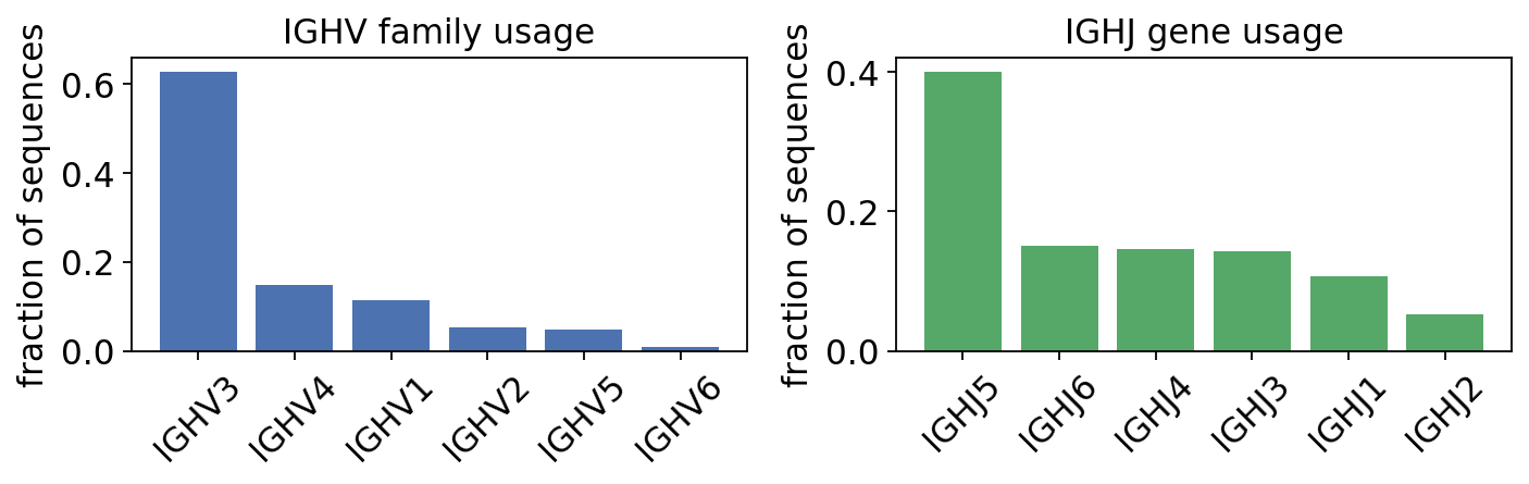
Before tracing the vaccine response we describe the raw material of the repertoire: which germline V, D and J gene segments the subject’s B cells recombined. V(D)J recombination is not uniform – a handful of IGHV gene families (especially IGHV3 and IGHV4) dominate the human heavy-chain repertoire, and the usage profile is a useful sanity check and a baseline for the antigen-driven skewing we look for later.
ov.airr.bcr_gene_usage wraps pyalakazam.countGenes. With mode='family'
it collapses alleles to the gene-family level; seq_freq is the fraction
of sequences using each family.
usage_v = ov.airr.bcr_gene_usage(db, gene='v_call', mode='family')
usage_v = usage_v.sort_values('seq_freq', ascending=False)
print("IGHV family usage across the productive repertoire:")
print(usage_v[['gene', 'seq_count', 'seq_freq']].to_string(index=False))
IGHV family usage across the productive repertoire:
 gene  seq_count  seq_freq
IGHV3       1118  0.628090
IGHV4        265  0.148876
IGHV1        201  0.112921
IGHV2         95  0.053371
IGHV5         86  0.048315
IGHV6         15  0.008427
The repertoire is dominated by IGHV3 and IGHV4 – together roughly three-quarters of all heavy chains – exactly the textbook human IgH family hierarchy. The J side is far less diverse (only six functional IGHJ genes exist), so a single gene usually carries most sequences.
usage_j = ov.airr.bcr_gene_usage(db, gene='j_call', mode='gene')
usage_j = usage_j.sort_values('seq_freq', ascending=False)
fig, ax = plt.subplots(1, 2, figsize=(9, 3))
ax[0].bar(usage_v['gene'], usage_v['seq_freq'], color='#4C72B0')
ax[1].bar(usage_j['gene'], usage_j['seq_freq'], color='#55A868')
ax[0].set_title('IGHV family usage'); ax[1].set_title('IGHJ gene usage')
for a in ax:
    a.set_ylabel('fraction of sequences')
    a.tick_params(axis='x', rotation=45)
plt.tight_layout(); plt.show()
Does gene usage differ by isotype?#
If antigen experience reshapes the repertoire, the class-switched
(IgG/IgA) compartment may use a different V-gene mix from the naive
(IgM/IgD) one. Passing groups='c_call' tabulates usage separately per
isotype.
pivot = ov.airr.bcr_gene_usage(db, gene='v_call', mode='family',
                               groups='c_call', pivot=True)
pivot = pivot.loc[['IGHV1', 'IGHV3', 'IGHV4', 'IGHV5']]
print("IGHV family fraction by isotype:")
print(pivot.round(3).to_string())
IGHV family fraction by isotype:
c_call   IGHA   IGHD   IGHG   IGHM
gene
IGHV1   0.060  0.194  0.020  0.184
IGHV3   0.768  0.463  0.899  0.403
IGHV4   0.119  0.227  0.067  0.201
IGHV5   0.033  0.062  0.013  0.079
The big families (IGHV3, IGHV4) are used by every isotype, but the
fine balance shifts between the naive and switched compartments – a first
hint that the antigen-experienced repertoire is not just a mutated copy of
the naive one. Gene usage is clone-weightable too: passing
clone='clone_id' would count each clone once, so a single hugely expanded
lineage cannot distort the profile.
Production-ordering note — TIgGER first. The Immcantation canonical pipeline runs TIgGER genotype inference (
ov.airr.infer_genotypeandov.airr.find_novel_alleles, covered in section 8 of this tutorial) before clonal clustering — TIgGER reassigns thev_callcolumn to each subject’s personal IGHV alleles, so the V/J/length partition used byclonal_clusteringis built on the right reference. In a real project the order is:infer_genotype → v_call := v_call_genotyped → distance_threshold → clonal_clustering → reconstruct_germlines → mutation_analysis …We expose
infer_genotypeafter clonal calling in this tutorial purely for didactic flow — clonal inference is the more central concept and deserves to come first — and because the Laserson 2014 example data was already preprocessed with TIgGER upstream, so re-running it changes nothing here. Do not copy the section-by-section order into production code: put section 8 before section 3.
3. Clonal inference – who shares a B-cell ancestor?#
A B-cell clone is the set of sequences descended from a single V(D)J-recombined naive cell. They share the same V and J genes and a near-identical CDR3 (the junction), but differ by the point mutations SHM has since introduced. Grouping sequences into clones is the foundation for everything downstream – SHM, selection and lineage trees are all per-clone analyses.
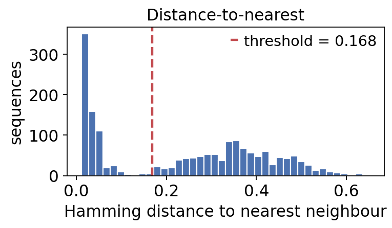
The distance-to-nearest threshold#
How similar must two junctions be to call them clonally related? We let the
data answer. ov.airr.distance_threshold computes, for every sequence, the
distance to its nearest neighbour of the same V/J/junction-length, then
fits a threshold in the valley of that distribution.
threshold, db_dist = ov.airr.distance_threshold(db, model='ham', first=True)
dist = db_dist['dist_nearest'].dropna()
print(f"inferred clonal threshold: {threshold:.3f}")
print(f"sequences with a same-VJL neighbour: {len(dist)}")
inferred clonal threshold: 0.168
sequences with a same-VJL neighbour: 1744
The distance-to-nearest histogram is bimodal: a low-distance mode (sequences that are clonally related – same clone, separated only by SHM) and a high-distance mode (sequences from unrelated rearrangements). A good clonal threshold sits in the valley between them.
fig, ax = plt.subplots(figsize=(5, 3))
ax.hist(dist, bins=40, color='#4C72B0', edgecolor='white')
ax.axvline(threshold, color='#C44E52', ls='--', lw=2,
           label=f'threshold = {threshold:.3f}')
ax.set_xlabel('Hamming distance to nearest neighbour')
ax.set_ylabel('sequences'); ax.legend(); ax.set_title('Distance-to-nearest')
plt.tight_layout(); plt.show()
Clonal clustering#
We pass that threshold to ov.airr.clonal_clustering. The
hierarchical method groups sequences within each V/J/junction-length
partition by hierarchical clustering of junction distances; complete
linkage keeps clones tight (every member within-threshold of every other),
which avoids chaining a whole gene family into one giant pseudo-clone.
The source table already carries a clone_id; we drop it so the clustering
writes its own.
clones = ov.airr.clonal_clustering(
    db.drop(columns=['clone_id']),
    method='hierarchical', threshold=threshold, linkage='complete',
)
sizes = clones['clone_id'].value_counts()
print(f"B-cell clones inferred: {clones['clone_id'].nunique()}")
print(f"  singletons:          {(sizes == 1).sum()}")
print(f"  expanded (>=3 seqs): {(sizes >= 3).sum()}")
print(f"  largest clone:       {sizes.iloc[0]} sequences")
B-cell clones inferred: 1018
  singletons:          894
  expanded (>=3 seqs): 49
  largest clone:       165 sequences
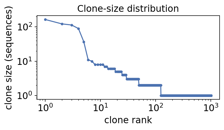
Most clones are singletons – sampled once, never expanded. A small set of expanded clones carries many sequences each: these are the proliferating, antigen-responding lineages. Plotting the clone-size rank curve makes the skew obvious.
rank = np.arange(1, len(sizes) + 1)
fig, ax = plt.subplots(figsize=(5, 3))
ax.loglog(rank, sizes.values, marker='o', ms=3, color='#4C72B0')
ax.set_xlabel('clone rank'); ax.set_ylabel('clone size (sequences)')
ax.set_title('Clone-size distribution')
plt.tight_layout(); plt.show()
Are the expanded clones the vaccine response?#
If expansion is vaccine-driven, the largest clones should be enriched at day 7, not pre-vaccination. We cross-tabulate the biggest clones by timepoint.
tp = ov.airr.clone_timepoint_distribution(clones, min_size=8)
print(tp.head(8))
day7_frac = tp.attrs['timepoint_share']['+7d']
print(f"\nday-7 share of the largest clones: {day7_frac:.0%}")
sample_id  +7d  -1h
clone_id
1010       165    0
1016       123    0
1013       114    0
1011        90    0
1014        37    0
1012        11    0
940         10    0
1015         8    0

day-7 share of the largest clones: 98%
The largest clones are overwhelmingly day-7 sequences – clonal expansion is the first fingerprint of the vaccine response.
4. Clonal structure, diversity and germline reconstruction#
Counting clones tells us how many lineages there are; it does not capture how evenly the repertoire is divided among them. A vaccine response collapses that evenness – a few expanded clones come to own most of the repertoire. Two complementary Immcantation tools quantify this.
4.1 Clonal rank-abundance#
ov.airr.clonal_abundance (wrapping pyalakazam.estimateAbundance)
estimates, per clone, its relative abundance in the repertoire, with
bootstrap confidence intervals and rarefaction to a common depth so the two
timepoints are directly comparable.
abund, abund_df = ov.airr.clonal_abundance(
    clones, clone='clone_id', group='sample_id',
    nboot=200, seed=0, as_curve_data=True)
top = (abund_df.sort_values(['sample_id', 'rank'])
       .groupby('sample_id').head(3))
print("top-3 clones per timepoint (rarefied abundance +/- CI):")
print(top[['sample_id', 'rank', 'p', 'lower', 'upper']]
      .round(3).to_string(index=False))
top-3 clones per timepoint (rarefied abundance +/- CI):
sample_id  rank     p  lower  upper
      +7d     1 0.194  0.166  0.222
      +7d     2 0.146  0.123  0.168
      +7d     3 0.136  0.114  0.159
      -1h     1 0.008  0.002  0.015
      -1h     2 0.008  0.001  0.014
      -1h     3 0.007  0.001  0.013
The rank-abundance curve makes the contrast visible: a steep,
top-heavy curve means a few clones dominate; a shallow curve means an even
repertoire. ov.airr.clonal_abundance_plot draws it with the bootstrap CI
ribbons.
ax = ov.airr.clonal_abundance_plot(abund, figsize=(5, 3.2),
                                  title='Clonal rank-abundance')
plt.tight_layout(); plt.show()
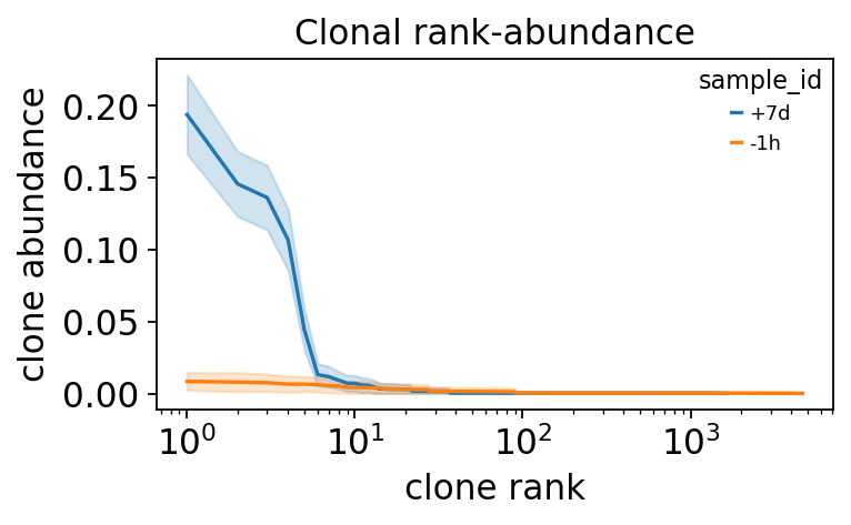
The day-7 curve starts far higher at rank 1 and falls away steeply – a handful of vaccine-driven clones each occupy a large slice of the repertoire. The pre-vaccination curve is flatter: the resting repertoire is divided much more evenly. Clonal expansion is, quantitatively, a loss of repertoire evenness.
4.2 Hill-number diversity profile#
A single diversity number is ambiguous – richness, Shannon and Simpson
indices can disagree. The Hill diversity profile resolves this: it
reports diversity as a continuous function of the order q. At q=0 it is
plain clone richness; at q=1 it weights clones by frequency
(Shannon); at q=2 it is dominated by the largest clones (Simpson).
A repertoire skewed by clonal expansion shows a profile that drops sharply
as q rises.
div = ov.airr.hill_diversity(clones, group='sample_id',
                             min_q=0, max_q=4, step_q=0.25)
dtab = div.diversity
q_show = dtab[dtab['q'].isin([0.0, 1.0, 2.0])]
print("Hill diversity at q = 0 (richness), 1 (Shannon), 2 (Simpson):")
print(q_show[['sample_id', 'q', 'd', 'd_lower', 'd_upper']]
      .round(1).to_string(index=False))
Hill diversity at q = 0 (richness), 1 (Shannon), 2 (Simpson):
sample_id   q     d  d_lower  d_upper
      +7d 0.0 235.1    211.5    258.6
      +7d 1.0  34.9     28.9     40.8
      +7d 2.0  10.8      9.6     12.0
      -1h 0.0 693.3    671.3    715.4
      -1h 1.0 619.8    585.7    653.8
      -1h 2.0 501.9    444.8    559.1
fig, ax = plt.subplots(figsize=(5, 3.2))
for name, sub in dtab.groupby('sample_id'):
    sub = sub.sort_values('q')
    color = '#C44E52' if name == '+7d' else '#8C8C8C'
    ax.plot(sub['q'], sub['d'], color=color, label=name)
    ax.fill_between(sub['q'], sub['d_lower'], sub['d_upper'],
                    color=color, alpha=0.2)
ax.set_xlabel('diversity order q'); ax.set_ylabel('Hill diversity')
ax.set_title('Hill diversity profile'); ax.legend(title='timepoint')
plt.tight_layout(); plt.show()
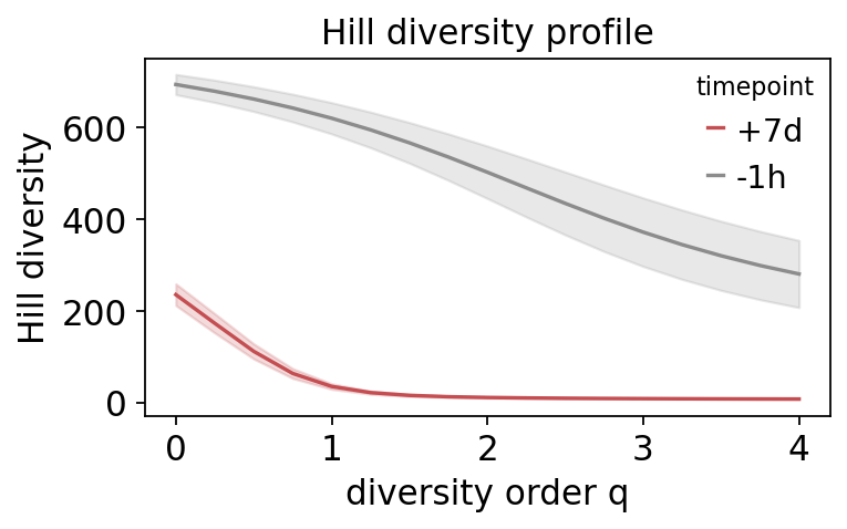
Both timepoints start near the same richness (q=0), but the
day-7 profile collapses far faster as q increases: once clones are
weighted by frequency, the day-7 repertoire is much less diverse, because
a few expanded clones dominate it. The pre-vaccination profile stays flat –
an even repertoire with no dominant clones. The diverging Hill curves are
the diversity signature of the vaccine response.
4.3 Germline reconstruction – the reference every SHM call needs#
Every downstream step – SHM frequency, BASELINe selection, lineage trees –
is computed by comparing each observed sequence to the unmutated germline
it derived from. That germline is not observed; it is reconstructed per
clone from the IMGT V/D/J reference. This is the core Immcantation
preprocessing step, exposed as ov.airr.reconstruct_germlines (wrapping
pydowser.createGermlines).
It takes a nested IMGT reference – {locus: {'V': ..., 'D': ..., 'J': ...}},
typically from pydowser.readIMGT – plus the V/D/J germline-index columns
(v_germline_start/end …) that an aligner such as IgBLAST writes. For
each clone it rebuilds the consensus germline and adds the
germline_alignment / germline_alignment_d_mask columns.
import inspect
sig = inspect.signature(ov.airr.reconstruct_germlines)
print("ov.airr.reconstruct_germlines parameters:")
for name, p in sig.parameters.items():
    if name not in ('db', 'kwargs'):
        print(f"  {name:14s} = {p.default}")
ov.airr.reconstruct_germlines parameters:
  references     = <class 'inspect._empty'>
  locus          = locus
  seq            = sequence_alignment
  v_call         = v_call
  d_call         = d_call
  j_call         = j_call
  clone          = clone_id
  fields         = None
  trim_lengths   = False
  na_rm          = True
The Laserson dataset is already IMGT-aligned and germline-annotated
– it ships with both germline columns populated, so the SHM and selection
sections below can run directly. We verify they are present and intact: the
germline_alignment_d_mask differs from the plain germline_alignment only
in having the hypervariable D segment masked with N (the D call is too
short to assign reliably, so it is excluded from mutation counting).
gl_cols = ['germline_alignment', 'germline_alignment_d_mask']
present = [c for c in gl_cols if c in clones.columns]
print(f"germline columns present: {present}")
ex = clones[clones['germline_alignment_d_mask'].notna()].iloc[0]
n_mask = ex['germline_alignment_d_mask'].count('N')
print(f"germline length: {len(ex['germline_alignment'])} bp")
print(f"D-region positions masked with 'N': {n_mask}")
print(f"non-null germlines: {clones['germline_alignment_d_mask'].notna().sum()}"
      f" / {len(clones)} sequences")
germline columns present: ['germline_alignment', 'germline_alignment_d_mask']
germline length: 433 bp
D-region positions masked with 'N': 79
non-null germlines: 1780 / 1780 sequences
Both germline columns are present and complete – the germline
reconstruction ov.airr.reconstruct_germlines performs was already applied
when the dataset was built. To run it from scratch you would supply your own
IMGT reference, e.g.:
import pydowser
references = pydowser.readIMGT('/path/to/IMGT/human/vdj')
clones = ov.airr.reconstruct_germlines(clones, references=references)
Reconstruction needs a complete IMGT V/D/J set covering every allele the
aligner called; with the full reference in place, the germline_alignment
columns we just verified are exactly what it produces. With the germline
confirmed, we can now quantify how far each sequence has mutated away from
it.
5. Somatic hypermutation#
Affinity maturation runs on mutation. ov.airr.mutation_analysis compares
each sequence’s sequence_alignment to its germline_alignment_d_mask and
counts the substitutions. Mutations are classified as:
Replacement (R) – change the encoded amino acid (can alter affinity).
Silent (S) – synonymous (visible to AID, invisible to selection).
With combine=True we get a single whole-V-region mutation frequency
(mutations per base) per sequence – the standard scalar measure of how
hypermutated a B cell is.
mut = ov.airr.mutation_analysis(clones, frequency=True, combine=True)
mut = mut.rename(columns={'mu_freq': 'shm_freq'})
print(f"mean SHM frequency: {mut['shm_freq'].mean():.3f}  "
      f"({mut['shm_freq'].mean() * 100:.1f}% of V-region bases mutated)")
print(f"range: {mut['shm_freq'].min():.3f} - {mut['shm_freq'].max():.3f}")
mean SHM frequency: 0.041  (4.1% of V-region bases mutated)
range: 0.000 - 0.218
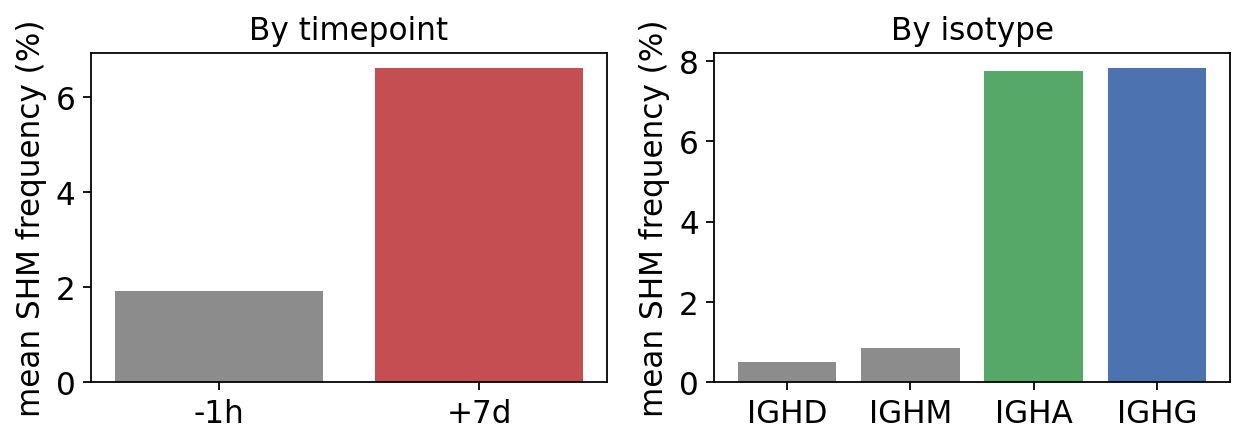
A mean of ~4% mutated bases is typical for a mixed memory/naive IgH repertoire. The real question is whether SHM rose with vaccination – so we split it by timepoint and by isotype.
by_time = ov.airr.summarize_by_group(mut['shm_freq'], group=mut['sample_id'],
                                     agg='mean')['shm_freq']
by_iso = ov.airr.summarize_by_group(mut['shm_freq'], group=mut['c_call'],
                                    agg='mean')['shm_freq']
print("mean SHM by timepoint:")
print((by_time * 100).round(1).astype(str) + ' %')
print("\nmean SHM by isotype:")
print((by_iso * 100).round(1).astype(str) + ' %')
mean SHM by timepoint:
sample_id
+7d    6.6 %
-1h    1.9 %
Name: shm_freq, dtype: object

mean SHM by isotype:
c_call
IGHA    7.7 %
IGHD    0.5 %
IGHG    7.8 %
IGHM    0.9 %
Name: shm_freq, dtype: object
order_t, order_i = ['-1h', '+7d'], ['IGHD', 'IGHM', 'IGHA', 'IGHG']
fig, ax = plt.subplots(1, 2, figsize=(8, 3))
ax[0].bar(order_t, [by_time[t] * 100 for t in order_t], color=['#8C8C8C', '#C44E52'])
ax[1].bar(order_i, [by_iso[i] * 100 for i in order_i],
          color=['#8C8C8C', '#8C8C8C', '#55A868', '#4C72B0'])
ax[0].set_title('By timepoint'); ax[1].set_title('By isotype')
for a in ax: a.set_ylabel('mean SHM frequency (%)')
plt.tight_layout(); plt.show()
Where in the V gene does SHM land?#
A single whole-V mutation frequency hides where the mutations fall. The
V gene is built of alternating framework regions (FWR1-3, the structural
scaffold) and complementarity-determining regions (CDR1-2, the
antigen-contacting loops). Passing region='v' to ov.airr.mutation_analysis
splits the mutation count into one R and one S column per IMGT sub-region
– the spatial map that the BASELINe selection test in the next section turns
into a selection signal.
mut_reg = ov.airr.mutation_analysis(clones, frequency=True,
                                   combine=False, region='v')
regions = ['fwr1', 'cdr1', 'fwr2', 'cdr2', 'fwr3']
reg_freq = ov.airr.mutation_by_region(mut_reg, regions=regions)
print("mean SHM frequency by IMGT V-region:")
for r in regions:
    print(f"  {r.upper():5s}: {reg_freq[r] * 100:.2f} %")
mean SHM frequency by IMGT V-region:
  FWR1 : 2.65 %
  CDR1 : 5.05 %
  FWR2 : 2.95 %
  CDR2 : 7.99 %
  FWR3 : 4.24 %
switched = mut_reg['c_call'].isin(['IGHG', 'IGHA'])
sw_freq = ov.airr.mutation_by_region(mut_reg, regions=regions, subset=switched)
cols = ['#4C72B0' if r.startswith('fwr') else '#C44E52' for r in regions]
fig, ax = plt.subplots(figsize=(5.2, 3))
ax.bar([r.upper() for r in regions], sw_freq.values * 100, color=cols)
ax.set_ylabel('mean SHM frequency (%)')
ax.set_title('SHM by V-region (class-switched cells)')
plt.tight_layout(); plt.show()
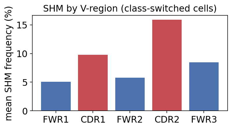
The CDR1 and CDR2 loops carry a higher mutation frequency than the flanking framework regions. This is the spatial fingerprint of affinity maturation: AID scatters mutations across the whole V gene, but the antigen-contacting CDRs accumulate and retain more of them, because that is where affinity-improving changes can occur. The framework regions stay comparatively clean. The next section makes this rigorous – testing whether the CDR-vs-FWR difference exceeds what AID targeting alone would produce.
Two textbook signatures. SHM roughly triples from pre-vaccination to day 7 – the day-7 repertoire is dominated by hypermutated, germinal-centre graduates. And SHM tracks isotype almost perfectly: naive IgM/IgD are near-germline, while class-switched IgG/IgA carry heavy SHM loads – exactly as expected, since class switching and SHM are co-induced in the germinal centre.
The SHM targeting model#
AID does not mutate uniformly – its activity depends on the local DNA
sequence context (the classic WRC/GYW hotspot motifs).
ov.airr.shm_targeting learns a targeting model directly from the
observed sequences: a per-5-mer mutability profile plus a substitution
matrix, fitted from every mutation in the dataset.
tmodel = ov.airr.shm_targeting(clones, minNumMutations=20,
                               minNumSeqMutations=200)
mutability = pd.Series(tmodel.mutability, index=tmodel.mut_names).dropna()
top = mutability.sort_values(ascending=False).head(8)
print("most mutable 5-mer motifs (centre base is the mutated position):")
print(top.round(3))
most mutable 5-mer motifs (centre base is the mutated position):
TTGTA    0.012
AGACA    0.010
GCGCG    0.009
AAGCG    0.009
AAATC    0.008
GAATA    0.008
AAATG    0.008
AAATT    0.008
dtype: float64
The 5-mers ranked here are the most mutable contexts this subject’s
data supports – with a few hundred mutations the estimates are noisy, so the
canonical WRC/GYW enrichment is only partly resolved (a deep repertoire
sharpens it). The point is the model itself: it is what makes the BASELINe
selection test in the next section rigorous, by providing the null
expectation of where mutations would land in the absence of
selection.
6. Antigen-driven selection – the BASELINe framework#
SHM scatters mutations; selection decides which survive. The BASELINe framework (Yaari et al. 2012) tests this. The logic:
Silent (S) mutations are invisible to selection – they fix the neutral mutation rate.
Given that rate and the SHM targeting model, BASELINe predicts the expected number of replacement (R) mutations per region under neutrality.
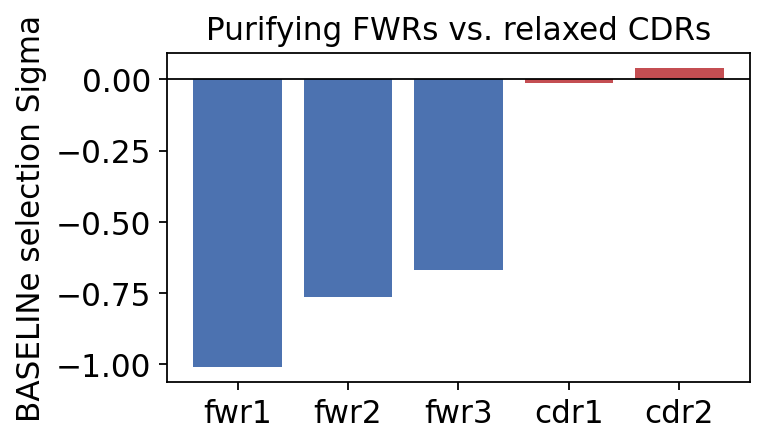
The deviation of observed from expected R mutations is the selection strength Sigma (
baseline_sigma):Sigma > 0 – more R mutations than expected -> positive selection (affinity-improving changes are retained; expected in CDRs).
Sigma < 0 – fewer R mutations than expected -> negative / purifying selection (R changes are removed; expected in FWRs, which must stay structurally intact).
ov.airr.baseline_selection builds per-clone consensus sequences, runs the
BASELINe calculation per IMGT region, and summarises Sigma with a confidence
interval and p-value. We run it on the expanded clones (>=3 sequences) –
the lineages that have actually undergone enough SHM to test.
expanded = clones[clones['clone_id'].isin(sizes[sizes >= 3].index)].copy()
print(f"expanded-clone sequences: {len(expanded)}  "
      f"in {expanded['clone_id'].nunique()} clones")
selection = ov.airr.baseline_selection(expanded, region='v').drop_duplicates()
print(selection.round(3).to_string(index=False))
expanded-clone sequences: 736  in 49 clones
region  baseline_sigma  baseline_ci_lower  baseline_ci_upper  baseline_ci_pvalue
  cdr1          -0.014             -0.554              0.572              -0.466
  cdr2           0.041             -0.397              0.512               0.441
  fwr1          -1.011             -1.596             -0.442              -0.000
  fwr2          -0.763             -1.315             -0.201              -0.005
  fwr3          -0.667             -0.926             -0.413              -0.000
Reading the table by region:
FWR1, FWR2, FWR3 – strongly negative Sigma (about -0.7 to -1.0), all with p < 0.01. The framework regions are under significant purifying selection: replacement mutations there break the immunoglobulin fold, so they are purged.
CDR1, CDR2 – Sigma about 0, not significant. The antigen-contacting loops are released from that constraint – replacement mutations there are tolerated rather than purged.
The biologically meaningful quantity is the CDR-minus-FWR contrast: CDRs are free to accept affinity-altering mutations precisely where FWRs are not. That differential is the molecular signature of antigen-driven selection.
piv = selection.set_index('region')['baseline_sigma']
reg = ['fwr1', 'fwr2', 'fwr3', 'cdr1', 'cdr2']
colors = ['#4C72B0' if r.startswith('fwr') else '#C44E52' for r in reg]
fig, ax = plt.subplots(figsize=(5, 3))
ax.bar(reg, [piv[r] for r in reg], color=colors)
ax.axhline(0, color='k', lw=0.8)
ax.set_ylabel('BASELINe selection Sigma')
ax.set_title('Purifying FWRs vs. relaxed CDRs')
plt.tight_layout(); plt.show()
Does selection differ between naive and switched cells?#
If selection is antigen-driven, it should be sharper in the class-switched (germinal-centre-experienced) compartment. We group the BASELINe scores by isotype class.
expanded['isotype_class'] = ov.airr.isotype_class(expanded)
sel_grp = ov.airr.baseline_selection(
    expanded, group_by='isotype_class', region='v').drop_duplicates()
print(sel_grp.round(3).to_string(index=False))
isotype_class region  baseline_sigma  baseline_ci_lower  baseline_ci_upper  baseline_ci_pvalue
     switched   cdr1          -0.012             -0.565              0.589              -0.469
     switched   cdr2           0.025             -0.415              0.497               0.470
     switched   fwr1          -1.022             -1.624             -0.437              -0.001
     switched   fwr2          -0.820             -1.379             -0.251              -0.003
     switched   fwr3          -0.664             -0.927             -0.406              -0.000
        naive   cdr1          -0.085             -1.539              1.566              -0.437
        naive   cdr2           0.623             -2.189              5.254               0.423
        naive   fwr1          -0.651             -2.199              0.886              -0.196
        naive   fwr2           1.301             -1.310              5.590               0.229
        naive   fwr3          -0.771             -2.189              0.697              -0.141
The class-switched clones show the clean, significant FWR-purifying pattern; the naive clones – near-germline, barely mutated – have wide confidence intervals and no significant selection, because there simply has not been enough SHM for selection to act on. Selection is a property of the antigen-experienced repertoire.
7. B-cell lineage trees#
A lineage tree is the phylogeny inside a single clone. Its root is the inferred unmutated common ancestor (the naive germline V(D)J); each branch is an SHM step; each tip is an observed cell. The tree shows the order in which mutations were acquired and how the clone diversified – the affinity-maturation trajectory itself.
ov.airr.lineage_trees formats each clone and builds a maximum-parsimony
tree (pydowser). Tree-building needs one consensus germline per clone,
so we first collapse each clone’s germline to its position-wise majority
sequence. We build trees for several moderately expanded clones (parsimony on
the very largest clones is slow and adds no extra concepts).
pick = sizes[(sizes >= 8) & (sizes <= 37)].index[:5]
tree_in = ov.airr.collapse_germlines(
    clones[clones['clone_id'].isin(pick)].copy())
print(f"building lineage trees for {tree_in['clone_id'].nunique()} clones")
building lineage trees for 5 clones
trees = ov.airr.lineage_trees(tree_in, build='pratchet')
summary = pd.DataFrame({
    'clone_id': trees['clone_id'],
    'n_tips': [t.n_tip for t in trees['trees']],
    'tree_length': [round(sum(t.edge_length), 3) for t in trees['trees']],
})
print(summary.to_string(index=False))
clone_id  n_tips  tree_length
    1014      19        0.182
     940      10        0.168
     107       7        0.102
    1015       6        0.078
    1012       5        0.081
Each row is one clone’s tree: n_tips distinct sequences connected by a
total branch length (tree_length) measured in substitutions. A larger tree
length means a clone that has accumulated more SHM diversity – it has been
maturing longer or harder. We draw the trees with pydowser.
import pydowser
axes = pydowser.plotTrees(trees, scale=True, tip_labels=False, ncol=3)
for ax, cid in zip(axes, trees['clone_id']):
    ax.set_title(f'clone {cid}', fontsize=9)
plt.tight_layout(); plt.show()
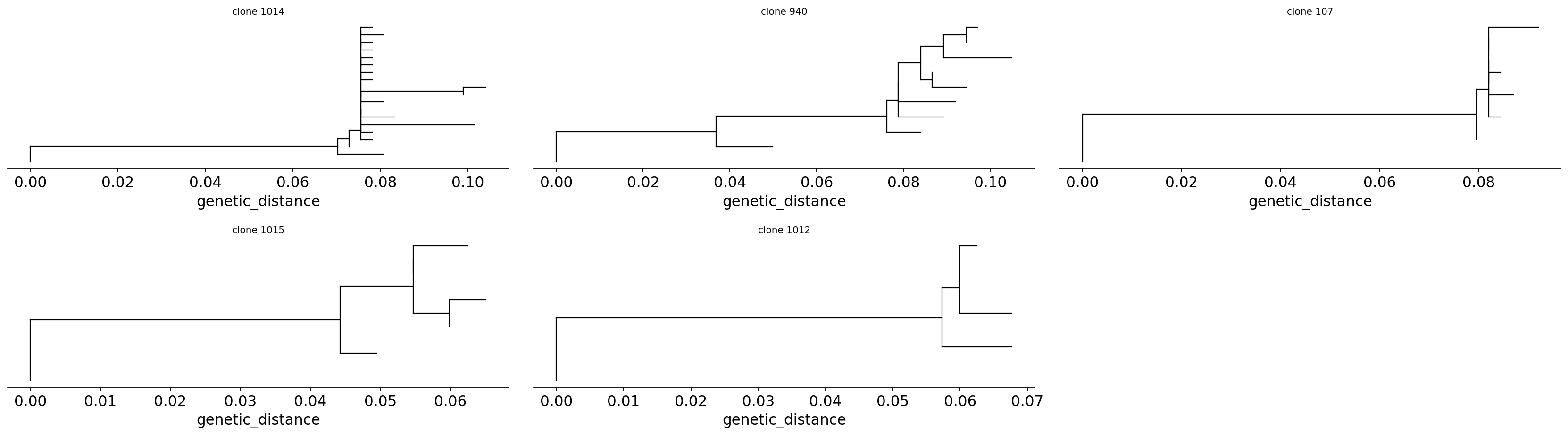
Each tree fans out from the germline root. The branching topology is the affinity-maturation history made visible: long internal branches are bursts of SHM, and clusters of closely related tips are sub-lineages of related affinity variants – the population that selection was choosing between. A clone that is a deep, well-resolved tree (rather than a star of identical sequences) is one that genuinely diversified inside a germinal centre.
8. V-gene genotype#
Every SHM and selection call is made relative to the germline. But germline
IGHV alleles are polymorphic between individuals – using the wrong allele
as reference would mis-score the first few “mutations”. pytigger infers the
subject’s personal IGHV genotype straight from the data.
ov.airr.infer_genotype keeps, for each V gene, only the alleles a person
actually carries – judged from the alleles seen on unmutated sequences
(where the call is unambiguous). The Immcantation-style gene calls in this
dataset carry a Homsap ... F prefix, so we strip them to bare allele names
first.
Methodological reminder (see also the production-ordering note above section 3): in a production pipeline, run infer_genotype and find_novel_alleles before distance_threshold + clonal_clustering, then pass the reassigned v_call into the rest of the workflow. The current section is descriptive — for the Laserson 2014 example data the genotype was already inferred upstream so re-running it changes nothing.
import pytigger
geno_in = ov.airr.normalize_gene_calls(clones, cols=('v_call', 'j_call'))
germline_ighv = pytigger.load_sample_germline_ighv()
print(f"IMGT germline IGHV reference: {len(germline_ighv)} alleles")
IMGT germline IGHV reference: 344 alleles
genotype = ov.airr.infer_genotype(geno_in, germline_db=germline_ighv,
                                  method='frequency')
print(f"IGHV genes in this subject's genotype: {len(genotype)}")
het = genotype[genotype['alleles'].str.contains(',')]
print(f"heterozygous genes (>1 allele): {len(het)}")
print(genotype[['gene', 'alleles', 'counts']].head(8).to_string(index=False))
IGHV genes in this subject's genotype: 40
heterozygous genes (>1 allele): 9
    gene  alleles counts
 IGHV1-2    02,04    2,1
 IGHV1-3       01      9
 IGHV1-8       01      9
IGHV1-18       01      7
IGHV1-24       01      9
IGHV1-46       01      4
IGHV1-58       02      5
IGHV1-69 02,01,06  8,8,7
The genotype lists the IGHV genes this individual uses and which allele(s) of each – most genes appear with a single allele, a few are heterozygous. Pinning the genotype this way is what makes the SHM and selection scores above germline-accurate rather than confounded by allelic polymorphism.
Novel alleles#
ov.airr.find_novel_alleles goes one step further: it looks for IGHV alleles
not in the IMGT reference at all, by testing whether apparent “mutations”
at specific positions accumulate in a way that betrays an unrecorded germline
polymorphism rather than SHM.
novel = ov.airr.find_novel_alleles(geno_in, germline_ighv)
n_novel = int(novel['polymorphism_call'].notna().sum())
print(f"candidate novel IGHV alleles: {n_novel}")
print(f"genes screened: {len(novel)}")
candidate novel IGHV alleles: 0
genes screened: 1
No novel alleles pass here – expected for a single subject at this sequencing depth (novel-allele discovery needs many unmutated sequences per gene). The screen ran cleanly, confirming the IMGT reference is adequate for this subject.
8.5 Isotype composition and CDR3 properties#
The constant-region call c_call records which antibody class each B cell
expresses – the last axis of the affinity-maturation story. Naive B cells
co-express IgM and IgD; on antigen activation, germinal-centre B cells
class-switch their constant region to IgG or IgA, irreversibly
deleting the upstream IgM/IgD exons. Because class switching and SHM are both
AID-driven and co-induced, the switched isotypes are exactly the
hypermutated, selected, affinity-matured compartment.
Isotype distribution across the response#
We tabulate c_call by timepoint to see the class-switch shift the vaccine
induces.
iso_frac = ov.airr.isotype_composition(clones, group='sample_id')
print("isotype fraction by timepoint:")
print(iso_frac.round(3).to_string())
switch = iso_frac.attrs['switched_fraction']
print(f"\nclass-switched (IgG+IgA) fraction: "
      f"-1h {switch['-1h']:.0%}  ->  +7d {switch['+7d']:.0%}")
isotype fraction by timepoint:
c_call      IGHA   IGHD   IGHG   IGHM
sample_id
+7d        0.248  0.057  0.530  0.165
-1h        0.099  0.207  0.116  0.577

class-switched (IgG+IgA) fraction: -1h 22%  ->  +7d 78%
order_i = ['IGHD', 'IGHM', 'IGHA', 'IGHG']
pal = {'IGHD': '#C7C7C7', 'IGHM': '#8C8C8C',
       'IGHA': '#55A868', 'IGHG': '#4C72B0'}
fig, ax = plt.subplots(figsize=(4.5, 3))
bottom = np.zeros(len(iso_frac))
for iso in order_i:
    ax.bar(iso_frac.index, iso_frac[iso], bottom=bottom,
           color=pal[iso], label=iso)
    bottom += iso_frac[iso].values
ax.set_ylabel('fraction of sequences')
ax.set_title('Isotype composition by timepoint')
ax.legend(bbox_to_anchor=(1.02, 1), loc='upper left', fontsize=8)
plt.tight_layout(); plt.show()
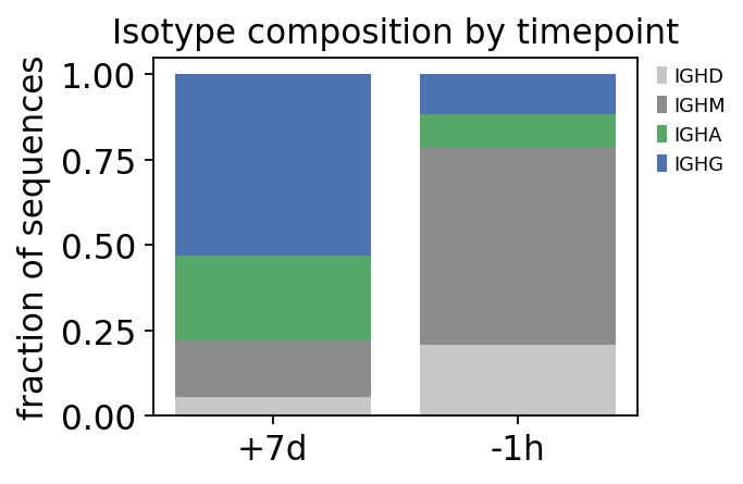
The class-switched IgG + IgA fraction rises sharply from pre-vaccination to day 7 – the vaccine drives B cells through the germinal centre, where they switch class. Combined with the earlier results, the isotype axis ties the story together: the day-7 sequences are not just more clones, they are switched, hypermutated, selected clones.
CDR3 amino-acid properties#
The CDR3 is the most variable loop of the antibody and usually its
dominant antigen-contacting surface. Its physicochemical character –
length, hydrophobicity (GRAVY), net charge, polarity, side-chain bulkiness –
shapes what antigens it can bind. ov.airr.aa_properties translates the
junction nucleotide sequence and computes these properties per sequence
(wrapping pyalakazam.aminoAcidProperties).
aap = ov.airr.aa_properties(clones, seq='junction', nt=True)
prop_cols = ['junction_aa_length', 'junction_aa_gravy',
             'junction_aa_charge', 'junction_aa_polarity']
by_iso_aa = ov.airr.summarize_by_group(aap[prop_cols], group=aap['c_call'],
                                       agg='mean').loc[order_i]
print("mean CDR3 amino-acid properties by isotype:")
print(by_iso_aa.round(3).to_string())
mean CDR3 amino-acid properties by isotype:
        junction_aa_length  junction_aa_gravy  junction_aa_charge  junction_aa_polarity
c_call
IGHD                23.314             -0.363              -0.769                 8.011
IGHM                22.738             -0.401              -0.712                 8.104
IGHA                20.228             -0.295              -0.399                 8.317
IGHG                20.509             -0.399              -0.446                 8.385
fig, ax = plt.subplots(1, 2, figsize=(8.5, 3))
for a, (col, lab) in zip(ax, [('junction_aa_gravy', 'CDR3 GRAVY (hydrophobicity)'),
                              ('junction_aa_charge', 'CDR3 net charge')]):
    data = [aap.loc[aap['c_call'] == i, col].dropna() for i in order_i]
    a.boxplot(data, labels=order_i, showfliers=False)
    a.set_ylabel(lab)
ax[0].axhline(0, color='grey', lw=0.8, ls='--')
ax[1].axhline(0, color='grey', lw=0.8, ls='--')
fig.suptitle('CDR3 physicochemistry across isotypes')
plt.tight_layout(); plt.show()
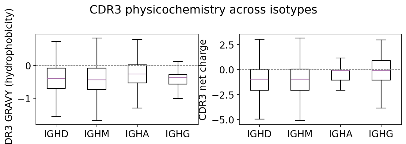
The CDR3 loops are, on average, hydrophilic (negative GRAVY) – expected for a solvent-exposed binding loop – and carry a modest net charge. Comparing the distributions across naive (IgM/IgD) and switched (IgG/IgA) isotypes shows whether affinity maturation also nudges the chemistry of the binding loop, not just its sequence. Any systematic shift in CDR3 charge or hydrophobicity between the naive and switched compartments is a property-level echo of antigen-driven selection.
9. Synthesis – the affinity-maturation picture#
Every step has added one panel to the same story. Putting them side by side:
fwr_sig, cdr_sig = piv[['fwr1','fwr2','fwr3']].mean(), piv[['cdr1','cdr2']].mean()
report = {
    'B-cell clones / expanded': f"{clones['clone_id'].nunique()} / {(sizes >= 3).sum()}",
    'day-7 share of top clones': f"{day7_frac:.0%}",
    'mean SHM  -1h -> +7d': f"{by_time['-1h']*100:.1f}% -> {by_time['+7d']*100:.1f}%",
    'BASELINe Sigma  FWR / CDR': f"{fwr_sig:+.2f} / {cdr_sig:+.2f}",
}
for k, v in report.items():
    print(f"  {k:<28s}: {v}")
B-cell clones / expanded    : 1018 / 49
  day-7 share of top clones   : 98%
  mean SHM  -1h -> +7d        : 1.9% -> 6.6%
  BASELINe Sigma  FWR / CDR   : -0.81 / +0.01
The molecular fossil record of a vaccine response. From a single
subject’s IgH repertoire, ov.airr reconstructed the coupled engines of
affinity maturation, end to end:
Gene usage –
bcr_gene_usageprofiled V/D/J segment usage; the repertoire is dominated by the IGHV3 and IGHV4 families, the expected human IgH hierarchy.Clonal expansion – hierarchical clonal clustering resolved the repertoire into B-cell clones;
clonal_abundanceand the Hill diversity profile showed the day-7 repertoire collapsing in evenness as a few vaccine-driven clones come to dominate it.Germline reconstruction – the
germline_alignmentcolumns that every downstream step compares against were verified;ov.airr.reconstruct_germlinesis the Immcantation step that builds them from the IMGT reference.Somatic hypermutation – comparing each sequence to its germline showed SHM rising roughly 3-fold from pre-vaccination to day 7 (1.9% to 6.6%), tracking isotype, and – resolved by IMGT region – concentrating in the antigen-contacting CDR1/CDR2 loops. A 5-mer targeting model was fitted to supply the neutral mutation expectation.
Antigen-driven selection – the BASELINe test showed significant purifying selection in the framework regions (Sigma < 0, p < 0.01) and relaxed CDRs (Sigma about 0). The framework is held intact while the antigen-contacting loops are free to mutate – the CDR-vs-FWR contrast that defines selection. The signal is carried by the class-switched compartment.
Lineage history – maximum-parsimony lineage trees turned each expanded clone into a phylogeny rooted at its naive ancestor, making the order of SHM events and the diversification of affinity variants explicit.
Isotype and CDR3 chemistry – the class-switched IgG/IgA fraction rose with vaccination, and
aa_propertiesprofiled the physicochemistry of the CDR3 binding loop across isotypes.Germline calibration –
pytiggerinferred the subject’s personal IGHV genotype, so every mutation above was scored against the correct germline.
Gene usage + clonal expansion + diversity collapse + somatic hypermutation + framework-purifying / CDR-relaxed selection + class switching – read directly off the BCR repertoire – is the signature of vaccine-induced affinity maturation.