Protein structure of an omics target — fetch, visualize, and assess before you trust

Protein structure of an omics target — fetch, visualize, and assess before you trust#

ov.mol is the bridge from an omics result to molecular structure. A typical omicverse analysis ends with a target — a differential gene from ov.bulk, a marker from ov.single, a variant from ov.genetics. This tutorial takes one such target and answers the first structural question: what does it look like in 3D?

But a predicted structure is not a fact — it is a hypothesis with a per-residue confidence map. The single most common mistake is to analyse a predicted model uniformly. So this tutorial follows the EBI / AlphaFold-team model-confidence interpretation workflow: check pLDDT and PAE first, then decide which regions are safe to interpret.

The target. We use EGFR (epidermal growth factor receptor) — a canonical druggable oncogene — as if it had just been handed over by an upstream differential-expression analysis.

What you will do

Fetch the structure (AlphaFold DB)
Assess pLDDT — per-residue confidence — with the interactive 3D viewer
Assess PAE — inter-domain confidence
Identify the well-folded domain suitable for drug work
Paint variant positions onto the structure (the omics bridge)
Predict a mutant structure absent from AlphaFold DB (ESMFold)

Requires pip install 'omicverse[mol]'. The 3D views are py3Dmol — they render inline and persist in the exported HTML docs.

Rendering note. Inline 3D views below use py3Dmol, which emits an HTML/JavaScript block. JupyterLab applies a trust filter that strips scripts from any notebook it has not signed with your local key — so a notebook you cloned from the repo, or one that was executed by nbconvert, opens untrusted and the views show only the “3Dmol.js failed to load” warning even though the HTML is saved in the file. To restore the interactive 3D views, either re-execute the cells in your own kernel (auto-trusts the current session) or run jupyter trust /path/to/this/notebook.ipynb in a terminal. The mkdocs-rendered version of this tutorial is static HTML, so the views work without trust there.

0. Setup#

import omicverse as ov
import numpy as np
import matplotlib.pyplot as plt
ov.plot_set()

🔬 Starting plot initialization...
🧬 Detecting GPU devices…
🚫 No GPU devices found (CUDA/MPS/ROCm/XPU)

   ____            _     _    __                  
  / __ \____ ___  (_)___| |  / /__  _____________ 
 / / / / __ `__ \/ / ___/ | / / _ \/ ___/ ___/ _ \ 
/ /_/ / / / / / / / /__ | |/ /  __/ /  (__  )  __/ 
\____/_/ /_/ /_/_/\___/ |___/\___/_/  /____/\___/                                              

🔖 Version: 2.2.1rc1   📚 Tutorials: https://omicverse.readthedocs.io/
✅ plot_set complete.

1. Fetch the target structure#

fetch_structure accepts a gene symbol, a UniProt accession or a PDB ID. Given a gene symbol it resolves gene → UniProt, then pulls the AlphaFold DB predicted model — which covers essentially every human protein, so any omics target has a structure to start from.

The returned MolStructure carries the parsed atoms, the one-letter sequence, and — crucially for a predicted model — the pLDDT confidence array and the PAE matrix.

s = ov.mol.fetch_structure('EGFR', verbose=True)
s

resolved gene EGFR -> UniProt P00533
fetched AlphaFold model AF-P00533-F1 (v6)

MolStructure(EGFR, source=alphafold, 1210 residues, mean pLDDT 75.9)

print(f'source        : {s.source}')
print(f'UniProt        : {s.uniprot}   gene: {s.gene}')
print(f'residues       : {s.n_residues}')
print(f'mean pLDDT     : {np.mean(s.plddt):.1f}')
print(f'PAE matrix     : {s.pae.shape}')

source        : alphafold
UniProt        : P00533   gene: EGFR
residues       : 1210
mean pLDDT     : 75.9
PAE matrix     : (1210, 1210)

2. pLDDT — per-residue confidence#

pLDDT is AlphaFold’s per-residue self-confidence (0–100). The AlphaFold team defines four bands:

Band	pLDDT	Interpretation
Very high	> 90	backbone and side chains reliable
High	70–90	backbone reliable
Low	50–70	treat with caution
Very low	< 50	likely disordered — not a folding failure, but a real prediction of disorder

Colour the structure by pLDDT — blue = confident, orange = unreliable. The view below is interactive: drag to rotate, scroll to zoom.

v = ov.mol.view(s, color_by='pLDDT', width=720, height=520)
v

ov.mol.view: pLDDT confidence bands (blue high -> orange low)

3Dmol.js failed to load for some reason. Please check your browser console for error messages.

<py3Dmol.view at 0x7f4dd0187fd0>

Quantify how much of the model falls in each band — this tells you, up front, how much of the protein you can actually interpret.

p = s.plddt
bands = {'Very high (>90)': p > 90, 'High (70-90)': (p > 70) & (p <= 90),
         'Low (50-70)': (p > 50) & (p <= 70), 'Very low (<=50)': p <= 50}
for name, mask in bands.items():
    print(f'{name:18s}: {100 * mask.mean():5.1f}%  ({mask.sum()} residues)')

Very high (>90)   :  47.2%  (571 residues)
High (70-90)      :  23.5%  (284 residues)
Low (50-70)       :   6.5%  (79 residues)
Very low (<=50)   :  22.8%  (276 residues)

EGFR is a large multi-domain receptor. A substantial low / very-low pLDDT fraction is expected — it is the flexible inter-domain linkers and the disordered C-terminal tail, not a broken model. The folded domains themselves score high.

3. PAE — is the domain arrangement trustworthy?#

pLDDT is local. It does not tell you whether two confidently-folded domains are placed correctly relative to each other. That is what PAE (Predicted Aligned Error) answers: PAE[i, j] is the expected error in residue i when the model is aligned on residue j.

Low PAE block on the diagonal → a well-defined domain.
High PAE between two diagonal blocks → the two domains are each confident, but their relative orientation is uncertain.

The practical rule: structure-based drug work must stay within a single low-PAE domain — never reason across a high-PAE inter-domain boundary.

ax = ov.mol.plot_pae(s)
plt.show()

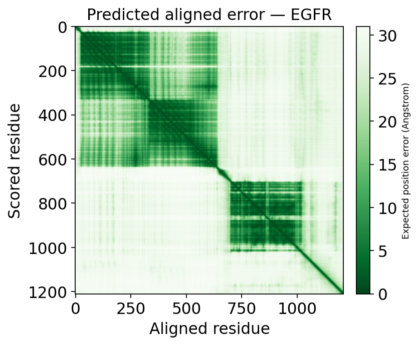
../_images/434fc9e1eb4b99b030124815805478d89a0da8c948801c53cd6b5356d3cd3c7b.png

The dark low-PAE blocks on the diagonal are EGFR’s individual domains. The bright off-diagonal regions are the inter-domain pairs whose relative arrangement AlphaFold is not confident about — exactly the boundaries not to reason across.

4. The well-folded domain for drug work#

EGFR’s intracellular tyrosine-kinase domain (UniProt residues ~712–979) is the drug target — every approved EGFR small-molecule inhibitor binds its ATP pocket. Confirm it is a high-confidence, well-folded region before doing any structural drug work on it.

rid = s.residue_ids
kinase = (rid >= 712) & (rid <= 979)
print(f'kinase domain (712-979): mean pLDDT {s.plddt[kinase].mean():.1f}'
      f'  over {kinase.sum()} residues')
print(f'rest of the protein     : mean pLDDT {s.plddt[~kinase].mean():.1f}')

kinase domain (712-979): mean pLDDT 84.1  over 268 residues
rest of the protein     : mean pLDDT 73.6

View just the kinase domain, coloured by confidence — this is the region the druggability and docking tutorials build on.

kin_residues = [int(r) for r in rid[kinase]]
v = ov.mol.view(s, color_by='pLDDT', highlight=None, width=720, height=520)
v

ov.mol.view: pLDDT confidence bands (blue high -> orange low)

3Dmol.js failed to load for some reason. Please check your browser console for error messages.

<py3Dmol.view at 0x7f4bbc9d5f60>

5. The omics bridge — paint variant positions#

This is where ov.mol earns its place in omicverse: a per-residue omics signal — variant calls from ov.genetics, a conservation track, a mutation-burden score — can be painted directly onto the 3D model.

EGFR has well-known oncogenic driver mutations. We highlight three canonical ones (UniProt / precursor numbering): G719S, T790M (“gatekeeper” resistance) and L858R (the most common activating mutation). highlight draws them as sticks on the cartoon.

variants = [719, 790, 858]
for pos in variants:
    i = int(np.where(rid == pos)[0][0])
    print(f'residue {pos} ({s.sequence[i]}): pLDDT {s.plddt[i]:.1f}')

residue 719 (G): pLDDT 73.3
residue 790 (T): pLDDT 88.4
residue 858 (L): pLDDT 51.2

Read the confidence at each variant before interpreting it:

G719 (pLDDT ≈ 73) and T790 (≈ 88) sit in well-folded, high-confidence regions — structural reasoning about those mutations stands on solid ground.
L858 scores pLDDT ≈ 51 — the low band. This is not a model failure: L858 lies in the kinase activation loop, a genuinely flexible element, and AlphaFold correctly reports low confidence there.

That is the workflow paying off: the same mutation list, but the model only supports confident structural claims for two of the three positions — for L858R, a rigid-structure argument must be made with caution. Now see where they fall in 3D:

v = ov.mol.view(s, color_by='pLDDT', highlight=variants,
                width=720, height=520)
v

ov.mol.view: pLDDT confidence bands (blue high -> orange low)

3Dmol.js failed to load for some reason. Please check your browser console for error messages.

<py3Dmol.view at 0x7f4bbc9d60e0>

The three highlighted residues cluster around the ATP-binding cleft — which is why they alter drug binding and drive resistance. The structure turns a flat list of variant positions into a mechanistic picture.

6. Predict a structure absent from AlphaFold DB#

AlphaFold DB stores the wild-type sequence. To see the mutant — or any sequence not in the database (a non-model species, a designed construct) — you must fold it yourself. predict_structure calls the ESMFold remote API: sequence → 3D, no MSA, no local GPU.

We build the L858R mutant of the EGFR kinase domain and fold it.

kin_seq = ''.join(c for r, c in zip(rid, s.sequence) if 712 <= r <= 979)
i858 = 858 - 712
mut_seq = kin_seq[:i858] + 'R' + kin_seq[i858 + 1:]
print(f'kinase domain: {len(kin_seq)} residues; '
      f'position 858 {kin_seq[i858]} -> {mut_seq[i858]}')

kinase domain: 268 residues; position 858 L -> R

mut = ov.mol.predict_structure(mut_seq, name='EGFR_L858R_kinase',
                               verbose=True)
print(f'{mut!r}  | mean pLDDT {np.mean(mut.plddt):.1f}')

MolStructure(?, source=esmfold, 268 residues, mean pLDDT 89.2)  | mean pLDDT 89.2

View the ESMFold-predicted mutant kinase domain, coloured by its own pLDDT. ESMFold reports confidence on the same 0–100 scale, so the four-band reading from step 2 applies identically.

v = ov.mol.view(mut, color_by='pLDDT', width=720, height=520)
v

ov.mol.view: pLDDT confidence bands (blue high -> orange low)

3Dmol.js failed to load for some reason. Please check your browser console for error messages.

<py3Dmol.view at 0x7f4bbc9d5420>

Interpretation#

A predicted structure is a hypothesis with a per-residue confidence map — pLDDT (local) and PAE (inter-domain). Always read both before interpreting a model.
Restrict structural drug work to a confident, low-PAE domain — for EGFR, the kinase domain.
The omics bridge — view(highlight=...), view(color_by=<score>) — only carries meaning where the model is confident.
For sequences absent from AlphaFold DB (mutants, designed constructs), predict_structure folds them on demand via ESMFold.

Next: the druggability tutorial detects the binding pockets of this kinase domain and asks whether the target is druggable.

Protein structure of an omics target — fetch, visualize, and assess before you trust

Contents

Protein structure of an omics target — fetch, visualize, and assess before you trust#

0. Setup#

1. Fetch the target structure#

2. pLDDT — per-residue confidence#

3. PAE — is the domain arrangement trustworthy?#

4. The well-folded domain for drug work#

5. The omics bridge — paint variant positions#

6. Predict a structure absent from AlphaFold DB#

Interpretation#