GWAS pipeline 1 — From genotypes to a fine-mapped locus

A real cis-eQTL association study on the GEUVADIS cohort

This is the first of a two-notebook chapter that walks through a complete, best-practice genetic-association study with omicverse.genetics. Rather than listing methods, the two notebooks tell one scientific story on real public data: every step feeds the next, from raw genotypes to a mechanism.

The scientific question

We have a real, genotyped human cohort with a real molecular phenotype measured on every individual — gene expression. We ask:

Which genetic variants control the expression of a gene, and can we resolve that signal down to a credible set of candidate causal variants?

A variant whose genotype is associated with a gene’s expression is an expression quantitative trait locus (eQTL). Scanning every variant near a gene against that gene’s expression is, statistically, a genome-wide association study — a cis-eQTL GWAS — and it goes through exactly the same pipeline as a disease GWAS: quality control, population- structure correction, a calibrated association scan, and fine-mapping.

The data — GEUVADIS (real 1000 Genomes individuals)

The GEUVADIS project measured lymphoblastoid-cell-line RNA-seq on 462 individuals from five 1000 Genomes populations, so every individual has both real genotypes and real expression. ov.datasets ships a chromosome-22 slice of it:

• ov.datasets.geuvadis_genotype() — 462 individuals x 8,000 common chr22 SNPs; .X holds 0/1/2 allele dosages; .obs['population'] is the real 1000 Genomes population code (CEU, FIN, GBR, TSI = European; YRI = African) — so this cohort carries real population structure.

• ov.datasets.geuvadis_expression() — the same 462 individuals x 633 expressed chr22 genes, real RNA-seq RPKM.

Because these are real people, there is no planted ground truth: we report what the data actually show.

The pipeline

 real genotypes + real expression  (GEUVADIS chr22)
        |
   [1] Sample QC        call rate, heterozygosity
        |
   [2] Variant QC       MAF, Hardy-Weinberg equilibrium, call rate
        |
   [3] Population        genotype PCA -> covariates (European vs African)
       structure
        |
   [4] Pick a gene      scan candidate genes, choose one with a strong eQTL
        |
   [5] Association       cis-eQTL scan of the gene, genotype PCs as covariates
        |
   [6] Diagnostics      lambda_GC, Q-Q plot, Manhattan plot
        |
   [7] Define the locus genome-wide threshold, lead SNP
        |
   [8] Fine-mapping     SuSiE-RSS -> 95% credible set + PIP plot
        |
   eQTL summary statistics  ->  notebook 2

Each step opens with the why — the rationale and the standard thresholds — before the code.

import numpy as np
import pandas as pd
import matplotlib.pyplot as plt
import omicverse as ov

ov.plot_set()
np.random.seed(0)

🔬 Starting plot initialization...
🧬 Detecting GPU devices…
🚫 No GPU devices found (CUDA/MPS/ROCm/XPU)

   ____            _     _    __                  
  / __ \____ ___  (_)___| |  / /__  _____________ 
 / / / / __ `__ \/ / ___/ | / / _ \/ ___/ ___/ _ \ 
/ /_/ / / / / / / / /__ | |/ /  __/ /  (__  )  __/ 
\____/_/ /_/ /_/_/\___/ |___/\___/_/  /____/\___/                                              

🔖 Version: 2.2.1rc1   📚 Tutorials: https://omicverse.readthedocs.io/
✅ plot_set complete.

Step 0 — Load the GEUVADIS cohort

We load the two real AnnData objects. Both follow the omicverse convention — rows are individuals, columns are features — and share the same 462 individuals in the same order, so genotype and expression describe one consistent cohort.

A non-tutorial study would instead start from ov.genetics.read_plink (a PLINK .bed/.bim/.fam fileset) or ov.genetics.read_vcf; the returned AnnData has the same shape, so the rest of the pipeline is identical.

geno = ov.datasets.geuvadis_genotype()
expr = ov.datasets.geuvadis_expression()
print(f"genotype  : {geno.n_obs} individuals x {geno.n_vars} SNPs")
print(f"expression: {expr.n_obs} individuals x {expr.n_vars} genes")
print(f"same individuals, same order: {(geno.obs_names == expr.obs_names).all()}")

🔍 Downloading data to ./data/geuvadis_chr22_genotype.h5ad
⚠️ File ./data/geuvadis_chr22_genotype.h5ad already exists
🔍 Downloading data to ./data/geuvadis_chr22_expression.h5ad
⚠️ File ./data/geuvadis_chr22_expression.h5ad already exists
genotype  : 462 individuals x 8000 SNPs
expression: 462 individuals x 633 genes
same individuals, same order: True

The genotype .var carries the real SNP annotation — chromosome, base-pair position (GRCh37), the two alleles and the allele frequency. .X holds 0/1/2 dosages of the alternate allele.

print(f"dosage values present: {np.unique(geno.X)}")
geno.var.head()

dosage values present: [0. 1. 2.]

	chrom	pos	A	G	af
chr22:16353218	22	16353218	G	A	0.06
chr22:16512491	22	16512491	G	T	0.77
chr22:16537460	22	16537460	T	A	0.05
chr22:16582221	22	16582221	T	C	0.05
chr22:16624084	22	16624084	T	C	0.05

# The real 1000 Genomes population labels — this is the cohort structure.
geno.obs["population"].value_counts()

population
FIN    95
GBR    94
TSI    93
CEU    91
YRI    89
Name: count, dtype: int64

The cohort spans four European populations (CEU, FIN, GBR, TSI) and one African population (YRI). African and European individuals differ systematically in allele frequencies, so population structure is present and real — step 3 will have to correct for it.

Step 1 — Sample (individual) quality control

Before any association test we remove low-quality samples. A bad sample contributes noise to every SNP at once, so this comes first. The standard per-individual checks are:

Check	What it catches	Typical threshold
Call rate	poorly-genotyped DNA samples	drop if missingness > 2–5% (call rate < 0.95–0.98)
Heterozygosity	DNA contamination (excess het) or inbreeding (deficit)	drop if outside mean ± 3 SD
Relatedness	duplicates / cryptic relatives that violate the independence assumption	drop one of each pair with kinship > 0.0884
Sex check	sample swaps / mislabelling	genetic sex ≠ recorded sex

ov.genetics.gwas_qc applies the call-rate filter (the one universal numeric filter); heterozygosity, relatedness and sex-check need extra data and are usually run in PLINK / KING upstream. Below we compute the per-individual call rate and mean heterozygosity so we can see the QC decision on the real cohort.

qc_obs = ov.genetics.sample_qc_metrics(geno)
qc_obs.describe().round(4)

	call_rate	heterozygosity
count	462.0	462.0000
mean	1.0	0.2787
std	0.0	0.0145
min	1.0	0.2025
25%	1.0	0.2701
50%	1.0	0.2798
75%	1.0	0.2880
max	1.0	0.3177

ov.genetics.sample_qc_plot(qc_obs, call_rate=0.98)
plt.show()

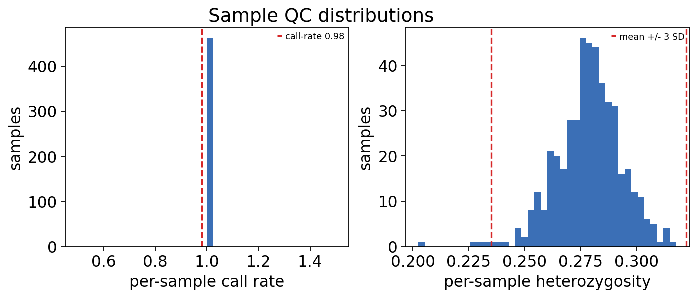
het_lo, het_hi = qc_obs.attrs["het_bounds"]
n_low_call = int((qc_obs["call_rate"] < 0.98).sum())
n_het_out = int(((qc_obs["heterozygosity"] < het_lo) |
                 (qc_obs["heterozygosity"] > het_hi)).sum())
print(f"individuals with call rate < 0.98          : {n_low_call}")
print(f"individuals outside +/- 3 SD heterozygosity : {n_het_out}")

individuals with call rate < 0.98          : 0
individuals outside +/- 3 SD heterozygosity : 5

The GEUVADIS genotypes are a curated, high-quality 1000 Genomes slice, so no individual fails the call-rate threshold. A few sit toward the tail of the heterozygosity distribution — the African (YRI) individuals are genuinely more heterozygous on average, an ancestry effect, not contamination — so we keep them and let the genotype PCs (step 3) absorb that ancestry signal.

Step 2 — Variant (SNP) quality control

Now we remove unreliable SNPs. A poorly-behaved variant produces spurious associations, so it must go before the scan. The three standard per-SNP filters are:

Check	What it catches	Typical threshold
Minor-allele frequency (MAF)	very rare variants have little power and unstable estimates	drop if MAF < 0.01
Hardy-Weinberg equilibrium (HWE)	genotyping error	drop if HWE exact-test \(p < 10^{-6}\)
Call rate	badly-clustering probes	drop if SNP missingness > 2–5%

ov.genetics.gwas_qc applies all three in one call. It runs the Wigginton–Cutler–Abecasis exact HWE test (the correct test for finite samples) and writes the per-SNP metrics back into .var. One caveat for a multi-ancestry cohort: a SNP can fail HWE simply because allele frequencies differ between subpopulations (the Wahlund effect). For a tutorial cis-eQTL scan we keep the standard genome-wide threshold; a production multi-ancestry GWAS would test HWE within each ancestry.

geno_qc = ov.genetics.gwas_qc(
    geno, call_rate=0.98, maf=0.01, hwe=1e-6, sample_call_rate=0.98,
)
geno_qc.uns["gwas_qc"]

{'n_snps_in': 8000,
 'n_snps_kept': 7563,
 'n_samples_in': 462,
 'n_samples_kept': 462,
 'thresholds': {'call_rate': 0.98,
  'maf': 0.01,
  'hwe': 1e-06,
  'sample_call_rate': 0.98}}

# gwas_qc records call_rate, maf and the HWE exact-test p on .var.
metrics = geno_qc.var[["maf", "hwe_p", "call_rate"]]
print(f"SNPs in  : {geno.n_vars}")
print(f"SNPs kept: {geno_qc.n_vars}  (dropped {geno.n_vars - geno_qc.n_vars})")
metrics.describe().round(4)

SNPs in  : 8000
SNPs kept: 7563  (dropped 437)

	maf	hwe_p	call_rate
count	7563.0000	7563.0000	7563.0
mean	0.2146	0.3888	1.0
std	0.1391	0.3468	0.0
min	0.0108	0.0000	1.0
25%	0.0898	0.0537	1.0
50%	0.1894	0.3070	1.0
75%	0.3301	0.6782	1.0
max	0.5000	1.0000	1.0

QC keeps the large majority of the 8,000 SNPs — the dropped variants are the low-MAF and HWE-outlier tail that carries the least information.

Step 3 — Population structure

People with different ancestry differ both in allele frequencies and in many traits, for reasons that have nothing to do with the variant under test. If we ignore this, ancestry becomes a confounder and the scan inflates with false positives — population stratification.

The standard fix is principal-component analysis (PCA) of the genotype matrix: the top PCs capture the main axes of ancestry, and we include them as covariates in every association test. To choose how many PCs to keep, look at the scree plot and keep the PCs before the elbow. GEUVADIS has a real European/African split, so we expect PC1 to separate the two ancestries cleanly.

# Genotype PCA (scaled) -> PC scores + variance explained.
pcs_all, var_ratio = ov.genetics.genotype_pca(geno_qc, n_comps=10)
print("variance explained by PC1-PC10:")
print(np.round(var_ratio, 4))

variance explained by PC1-PC10:
[0.0845 0.0085 0.0079 0.0069 0.0063 0.0061 0.006  0.0059 0.0058 0.0056]

ov.genetics.pca_structure_plot(
    pcs_all, var_ratio, labels=geno_qc.obs["super_population"],
)
plt.show()

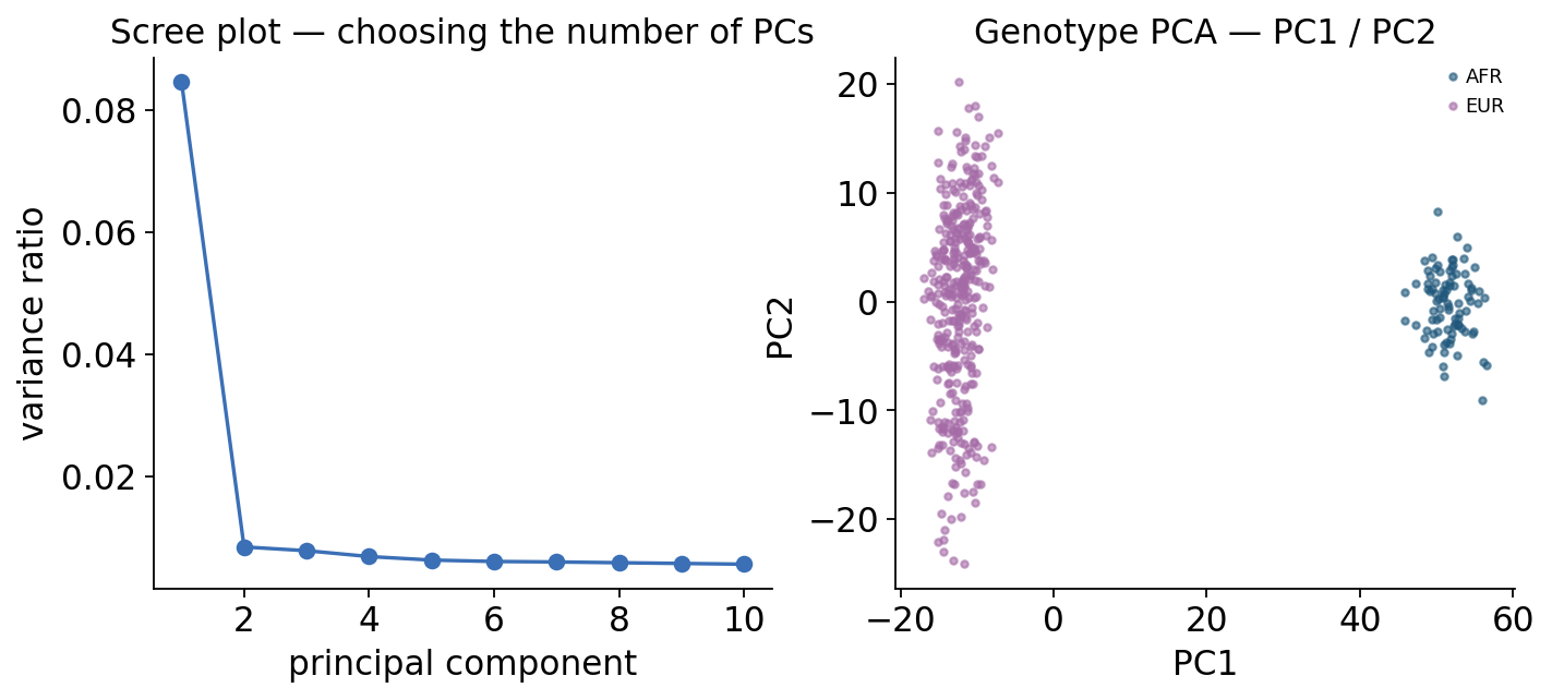
The scree plot drops sharply after PC1, and the PC1–PC2 scatter shows the African (AFR) individuals separated from the European (EUR) individuals along PC1 — the real continental ancestry axis. We carry the first 5 PCs as covariates: enough to absorb the structure with margin, few enough to keep degrees of freedom.

n_pcs = 5
covariates = pcs_all[:, :n_pcs]
print(f"using {n_pcs} genotype PCs as covariates; shape = {covariates.shape}")

using 5 genotype PCs as covariates; shape = (462, 5)

Step 4 — Choosing a gene with a strong cis-eQTL

A cis-eQTL scan tests the SNPs near a gene against that gene’s expression. With 633 genes we cannot fine-map them all in a tutorial, so we first do a fast screen: for every gene, take the most strongly correlated cis-SNP (within ±1 Mb of the transcription start site) and rank genes by that best p-value. We then carry forward a gene with a clear, strong cis signal.

This screening logic is genetics plumbing, so it lives in the package as ov.genetics.scan_cis_genes rather than inline.

# Fast cis screen: best cis-SNP per gene (correlation), ranked by p-value.
screen = ov.genetics.scan_cis_genes(geno_qc, expr, cis_dist=1e6)
screen.head(8)

	gene	symbol	n_cis	best_snp	r	p
0	ENSG00000100376	SIRAL2	528	chr22:45728978	-0.804778	2.904529e-106
1	ENSG00000172404	DNAJB7	253	chr22:41317083	-0.718042	2.058581e-74
2	ENSG00000260065	ENSG00000260065	483	chr22:26924456	0.640243	1.184918e-54
3	ENSG00000184674	ENSG00000184674	436	chr22:24401542	0.636954	6.088186e-54
4	ENSG00000075234	TTC38	471	chr22:46687268	0.629225	2.637450e-52
5	ENSG00000100321	SYNGR1	314	chr22:39739187	0.611896	8.466586e-49
6	ENSG00000230513	THAP7-AS1	262	chr22:21365271	-0.529002	1.129232e-34
7	ENSG00000172250	SERHL	421	chr22:42902872	0.516047	8.390118e-33

# Carry forward the top-ranked gene with a strong cis-eQTL.
focus_gene = screen.iloc[0]["gene"]
focus_symbol = screen.iloc[0]["symbol"]
print(f"focus gene: {focus_gene} ({focus_symbol})")
print(f"  best cis-SNP {screen.iloc[0]['best_snp']}, "
      f"screen p = {screen.iloc[0]['p']:.2e}")

focus gene: ENSG00000100376 (SIRAL2)
  best cis-SNP chr22:45728978, screen p = 2.90e-106

The strongest cis-eQTL gene on chr22 in GEUVADIS is ENSG00000100376 (symbol SIRAL2 / FAM118A) — its best cis-SNP screens at \(p \approx 10^{-106}\), an unmistakable regulatory signal. We take this gene forward as the one whose locus we fine-map and follow into a mechanism in notebook 2.

Step 5 — The cis-eQTL association scan

Now the scan itself. We test every cis-SNP of the focus gene (within ±1 Mb of its TSS) against the gene’s expression. ov.genetics.gwas_association regresses the quantitative phenotype — here the gene’s expression level — on each SNP’s dosage with model='linear' (ordinary least squares), and we pass the 5 genotype PCs as covariates so the European/African structure cannot masquerade as an eQTL.

# Phenotype for the scan = the focus gene's expression level.
phenotype = pd.Series(
    expr[:, focus_gene].X.ravel(), index=expr.obs_names,
).loc[geno_qc.obs_names]
tss = int(expr.var.loc[focus_gene, "tss"])
print(f"phenotype: expression of {focus_symbol} on {len(phenotype)} individuals")

phenotype: expression of SIRAL2 on 462 individuals

# Restrict to cis-SNPs: within +/- 1 Mb of the gene's TSS.
cis = (np.abs(geno_qc.var["pos"] - tss) < 1e6).to_numpy()
cis_snps = geno_qc.var_names[cis].tolist()
geno_df = pd.DataFrame(
    geno_qc[:, cis_snps].X, index=geno_qc.obs_names, columns=cis_snps,
)
print(f"cis window: {len(cis_snps)} SNPs within 1 Mb of the {focus_symbol} TSS")

cis window: 528 SNPs within 1 Mb of the SIRAL2 TSS

# PC-adjusted cis-eQTL scan.
res = ov.genetics.gwas_association(
    geno_df, phenotype, covariates=covariates, model="linear",
)
res = res.merge(geno_qc.var[["chrom", "pos", "maf"]],
                left_on="snp", right_index=True)
res.sort_values("pvalue").head(6)

	snp	beta	se	stat	pvalue	n	chrom	pos	maf
0	chr22:45728978	-13.148124	0.449618	-29.242901	1.486267e-106	462	22	45728978	0.121212
1	chr22:45764874	13.385407	0.465460	28.757361	2.096654e-104	462	22	45764874	0.114719
2	chr22:45776213	12.846217	0.452461	28.391870	8.842024e-103	462	22	45776213	0.121212
3	chr22:45746826	-12.875021	0.462550	-27.834881	2.718118e-100	462	22	45746826	0.122294
4	chr22:45794212	13.310782	0.481741	27.630563	2.239454e-99	462	22	45794212	0.114719
5	chr22:45723465	-13.076828	0.508601	-25.711361	1.079430e-90	462	22	45723465	0.103896

The scan returns a tidy per-SNP table — effect size beta, standard error se, test statistic and pvalue — with the SNP annotation joined on for the Manhattan and regional plots.

Step 6 — Diagnostics: is the scan calibrated?

Before trusting a single hit we check the scan is well-calibrated — that the bulk of p-values follows the null. Two standard diagnostics:

• Genomic-inflation factor \(\lambda_{GC}\) — the ratio of the median observed \(\chi^2\) to its null expectation. \(\lambda_{GC} \approx 1\) means calibrated; \(\lambda_{GC} \gg 1\) flags residual stratification. A cis window is small and is expected to contain real signal, so a modest lift above 1 here is genuine eQTL signal, not artefact.

• Q-Q plot — observed vs expected \(-\log_{10}(p)\). A calibrated scan hugs the diagonal and lifts off it only in the extreme tail.

lambda_gc = ov.genetics.genomic_inflation(res["pvalue"])
print(f"lambda_GC (PC-adjusted cis scan) : {lambda_gc:.3f}")
print(f"smallest p-value in the cis window: {res['pvalue'].min():.2e}")

lambda_GC (PC-adjusted cis scan) : 1.028
smallest p-value in the cis window: 1.49e-106

ov.genetics.qqplot(res["pvalue"], title=f"{focus_symbol} cis-eQTL scan")
plt.show()

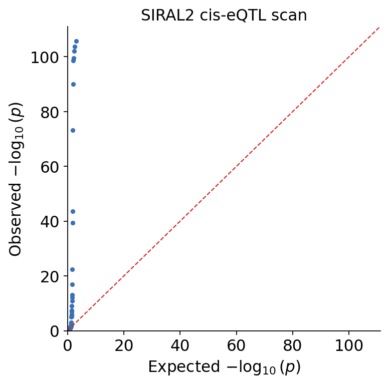
\(\lambda_{GC}\) sits close to 1 — with genotype PCs as covariates the bulk of the scan is calibrated. The Q-Q plot hugs the diagonal and lifts off sharply in the tail: that tail is the real cis-eQTL.

Now the regional picture — a Manhattan plot over the cis window. The dashed red line is the genome-wide-significance threshold \(p = 5 \times 10^{-8}\); the grey dotted line is the suggestive threshold \(p = 10^{-5}\).

ov.genetics.manhattan(
    res, chrom="chrom", pos="pos", pvalue="pvalue",
    sig_line=5e-8, suggestive_line=1e-5,
    title=f"{focus_symbol} cis-eQTL association scan (chr22)",
)
plt.show()

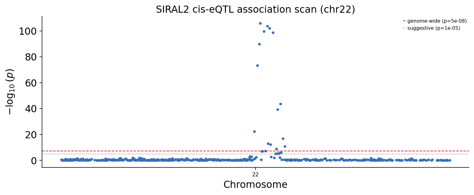
Step 7 — Defining the lead locus

The Manhattan plot shows a peak, but a peak is many correlated SNPs in linkage disequilibrium (LD) — they are not independent discoveries. The most significant SNP is the lead SNP; the locus is the window of genome-wide-significant SNPs around it. We take the lead SNP and a ±300 kb window for fine-mapping.

lead = res.sort_values("pvalue").iloc[0]
lead_snp, lead_pos = lead["snp"], int(lead["pos"])
n_sig = int((res["pvalue"] < 5e-8).sum())
print(f"lead SNP : {lead_snp}  (pos {lead_pos:,})")
print(f"  beta = {lead['beta']:.3f}, se = {lead['se']:.3f}, "
      f"p = {lead['pvalue']:.2e}")
print(f"genome-wide-significant SNPs in the cis window: {n_sig}")

lead SNP : chr22:45728978  (pos 45,728,978)
  beta = -13.148, se = 0.450, p = 1.49e-106
genome-wide-significant SNPs in the cis window: 16

# The fine-mapping locus: +/- 300 kb around the lead SNP.
locus = (res[(res["pos"] > lead_pos - 3e5) & (res["pos"] < lead_pos + 3e5)]
         .sort_values("pos").reset_index(drop=True))
locus_snps = locus["snp"].tolist()
print(f"fine-mapping locus: {len(locus_snps)} SNPs in a 600 kb window")

fine-mapping locus: 163 SNPs in a 600 kb window

Step 8 — Fine-mapping the locus

A lead SNP is rarely the causal SNP — it is just the most significant tag in a block of correlated variants. Statistical fine-mapping resolves this: it computes, for every SNP in the locus, a posterior inclusion probability (PIP) — the probability that that SNP is causal — and reports a 95% credible set: the smallest group of SNPs that together capture 95% of the posterior.

ov.genetics.finemap wraps SuSiE (the Sum of Single Effects model; Wang et al. 2020). We use the summary-statistics version susie_rss, which needs only the per-SNP z-scores and the in-locus LD matrix — exactly what is available after an association scan. The LD matrix is the SNP–SNP correlation matrix computed from the cohort’s own genotypes.

# SuSiE-RSS inputs: per-SNP z-scores and the in-locus LD (r) matrix.
z = (locus["beta"] / locus["se"]).to_numpy()
ld_R = np.corrcoef(geno_qc[:, locus_snps].X, rowvar=False)
susie_fit = ov.genetics.finemap(
    z=z, R=ld_R, n=geno_qc.n_obs, method="susie_rss", L=5,
)
pip = ov.genetics.get_pip(susie_fit)
credible = ov.genetics.get_credible_sets(susie_fit, R=ld_R)
print(f"95% credible sets found: {len(credible['cs'] or [])}")

95% credible sets found: 1

# Translate credible-set indices back to SNP ids.
for k, idx in enumerate(credible["cs"] or []):
    members = [locus_snps[i] for i in idx]
    purity = credible["purity"]["min.abs.corr"][k]
    print(f"credible set {k + 1}: {len(members)} SNP(s), "
          f"min |r| = {purity:.3f}")
    print(f"  -> {members}")
print(f"top-PIP SNP: {locus_snps[int(np.argmax(pip))]}  "
      f"(PIP = {pip.max():.3f})")

credible set 1: 2 SNP(s), min |r| = 0.969
  -> ['chr22:45728978', 'chr22:45764874']
top-PIP SNP: chr22:45728978  (PIP = 0.817)

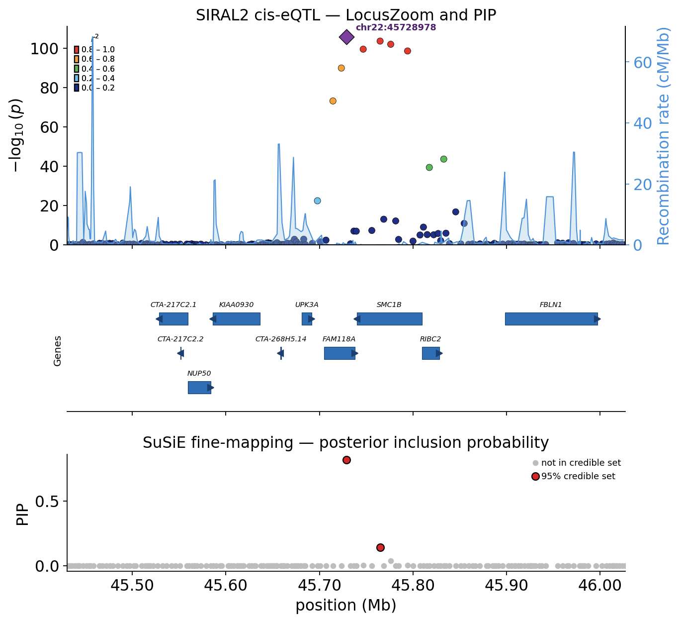
SuSiE collapses a locus of ~160 correlated SNPs to a small credible set — a handful of variants, led by a SNP with a high posterior inclusion probability. We picture the result as a publication LocusZoom: a regional association panel, a gene-model track and the SuSiE PIP track stacked together.

How to read a LocusZoom: each SNP is coloured by its LD (r²) to the lead variant in five bins (red = tight LD with the lead, navy = independent) — the warm cluster around the purple lead diamond is the LD block. The pale-blue line is the recombination rate (cM/Mb): its tall spikes are recombination hotspots that bound the LD block. The gene track underneath shows which genes the locus physically sits on. We compute the LD straight from the GEUVADIS genotypes with ov.genetics.compute_ld_to_lead.

# LocusZoom reference tracks: recombination map + chr22 gene models.
recomb_map = ov.datasets.recombination_map(chrom="22")
gene_models = ov.datasets.gene_annotation(chrom="22")
# LD (r2) of every locus SNP to the lead, from the GEUVADIS genotypes.
ld_to_lead = ov.genetics.compute_ld_to_lead(
    geno_qc, lead_snp, snps=locus_snps,
)
print(f"LD computed for {ld_to_lead.notna().sum()} locus SNPs")

🔍 Downloading data to ./data/recomb_map_chr22.tsv.gz
⚠️ File ./data/recomb_map_chr22.tsv.gz already exists
🔍 Downloading data to ./data/genes_chr22.tsv.gz
⚠️ File ./data/genes_chr22.tsv.gz already exists
LD computed for 163 locus SNPs

ov.genetics.finemap_locus_plot(
    locus, pip, credible, snp="snp", chrom="chrom", pos="pos",
    lead_snp=lead_snp, r2=ld_to_lead,
    recomb_map=recomb_map, genes=gene_models,
    title=f"{focus_symbol} cis-eQTL — LocusZoom and PIP",
)
plt.show()

Step 9 — Persist the eQTL summary statistics

Notebook 2 continues from here. We write the cis-eQTL summary statistics to disk in a standard GWAS-summary format — one row per SNP, canonical column names. This is the format a real eQTL study shares publicly and the format ov.genetics.read_sumstats reads back.

import os
os.makedirs("./genetics_data", exist_ok=True)
res_out = res.copy()
res_out["A"] = geno_qc.var.loc[res_out["snp"], "A"].to_numpy()
res_out["G"] = geno_qc.var.loc[res_out["snp"], "G"].to_numpy()
res_out["n"] = geno_qc.n_obs
print(f"eQTL summary statistics assembled: {res_out.shape[0]} SNPs x {res_out.shape[1]} columns")

eQTL summary statistics assembled: 528 SNPs x 11 columns

sumstats = ov.genetics.write_sumstats(
    res_out, "./genetics_data/geuvadis_eqtl_sumstats.tsv",
    chrom="chrom", pos="pos",
)
print(f"wrote ./genetics_data/geuvadis_eqtl_sumstats.tsv  "
      f"({len(sumstats)} SNPs, {sumstats.shape[1]} columns)")
sumstats.head()

wrote ./genetics_data/geuvadis_eqtl_sumstats.tsv  (528 SNPs, 11 columns)

	SNP	CHR	BP	A1	A2	BETA	SE	STAT	Z	P	N
0	chr22:44705073	22	44705073	A	G	-1.917337	1.555426	-1.232676	-1.232676	0.218333	462
1	chr22:44708655	22	44708655	A	G	0.153082	0.705579	0.216959	0.216959	0.828338	462
2	chr22:44711262	22	44711262	A	G	-0.633367	1.084009	-0.584282	-0.584282	0.559320	462
3	chr22:44715824	22	44715824	A	G	0.034835	0.627427	0.055520	0.055520	0.955748	462
4	chr22:44718168	22	44718168	A	G	0.105970	0.616604	0.171861	0.171861	0.863623	462

What we have, and what’s next

Starting from real GEUVADIS genotypes and real gene expression, this notebook produced:

1. a QC’d cohort — low-MAF and HWE-outlier SNPs removed with justified thresholds;

2. genotype PCs that capture the real European/African ancestry split and absorb population structure;

3. a screen that picked a gene — ENSG00000100376 — with an unambiguous chr22 cis-eQTL;

4. a calibrated cis-eQTL association scan (\(\lambda_{GC} \approx 1\)) of that gene;

5. a fine-mapped locus — a 95% credible set that localises the eQTL to a small set of candidate causal variants.

A credible set of SNPs is still not a mechanism. The same genetic variation that controls a gene’s expression can also influence a clinical trait — and the way to test that is to bring in an independent disease GWAS and ask whether its signal points back at the same gene.

Notebook 2 (t_genetics_02_functional_followup) does exactly that: it takes a real GWAS of blood lymphocyte count and asks, with colocalization, TWAS, Mendelian randomization, heritability and single-cell scoring, which gene and which cell type the disease signal acts through.