Joint single-cell TCR + gene-expression analysis — a CoNGA-style workflow

This tutorial walks the ov.airr TCR + GEX joint-analysis module — a clean, AnnData-native reimplementation of the core of CoNGA (“Clonotype Neighbor Graph Analysis”, Schattgen et al., Nat Biotechnol 2022). Where the earlier AIRR tutorials looked at the receptor or the transcriptome, this one asks how the two co-vary.

The two identities of a T cell, and why pairing them matters

Every T cell carries two pieces of information at once:

• its transcriptome — what state the cell is in (naive, effector, exhausted, memory);

• its T-cell receptor (TCR) — what clone it belongs to, and, indirectly, what antigen it can see.

These are assembled by completely different processes — V(D)J recombination fixes the receptor once, transcription is dynamic — so a priori they are statistically independent. A CoNGA-style analysis looks for the places where they are not independent: cells whose neighbours in transcriptome space are also their neighbours in TCR space. Such a coupling is the molecular fingerprint of an antigen-driven response — a clonally related group of T cells that have been pushed into a shared transcriptional program by recognising the same peptide.

The CoNGA idea: graph vs graph

CoNGA builds two kNN graphs over the same cells:

1. a GEX graph — nearest neighbours in the gene-expression embedding (obsm['X_pca']);

2. a TCR graph — nearest neighbours in TCR-sequence space (TCRdist, or a CDR3 Hamming fallback; cells of the same clonotype are always linked).

For every cell it then asks a simple question: do my two neighbourhoods overlap more than chance would allow? — scored with a hypergeometric test. Cells where the answer is yes are CoNGA hits: their transcriptional state and their receptor are locked together.

What this notebook covers

Section	ov.airr function	Question
3	conga_score	which cells show TCR ↔ GEX coupling?
4	conga_clusters	which (GEX-cluster × TCR-cluster) combinations are coherent?
5	tcr_clumping	which clonotypes converge in TCR space beyond a recombination background?
6	hotspot_features	which genes are localized on the graph?
7	synthesis	tie TCR specificity / antigen labels back to transcriptional state

0. Setup

The TCR + GEX joint module lives in ov.airr alongside the rest of the immune-repertoire suite. It is AnnData-native: the gene-expression matrix stays in adata.X, the GEX embedding in adata.obsm, and the per-cell receptor data in adata.obs — so a CoNGA-style analysis composes directly with the omicverse single-cell stack. Nothing here needs a separate object or an external single-cell library.

import omicverse as ov
import numpy as np
import pandas as pd
import matplotlib.pyplot as plt
ov.plot_set()
print("omicverse", ov.__version__)

🔬 Starting plot initialization...
🧬 Detecting GPU devices…
🚫 No GPU devices found (CUDA/MPS/ROCm/XPU)

   ____            _     _    __                  
  / __ \____ ___  (_)___| |  / /__  _____________ 
 / / / / __ `__ \/ / ___/ | / / _ \/ ___/ ___/ _ \ 
/ /_/ / / / / / / / /__ | |/ /  __/ /  (__  )  __/ 
\____/_/ /_/ /_/_/\___/ |___/\___/_/  /____/\___/                                              

🔖 Version: 2.2.1rc1   📚 Tutorials: https://omicverse.readthedocs.io/
✅ plot_set complete.

omicverse 2.2.1rc1

1. Load and inspect the antigen-labelled dataset

ov.datasets.airr_tcr_antigen() fetches the 10x Genomics dCODE dextramer experiment — CD8+ T cells from a healthy donor, profiled with paired 5′ scTCR-seq + gene expression and a panel of 44 pMHC dextramer reagents. A dextramer is a fluorescent multimer of a specific peptide–MHC complex: a T cell that binds one is, by construction, specific for that peptide. So this dataset comes with a ground-truth antigen label per cell — the ideal benchmark for asking whether TCR specificity predicts transcriptional state.

The tutorial subset is 6,500 cells × 2,012 genes, already carrying a precomputed PCA / UMAP embedding, a leiden GEX clustering, the per-cell ov.airr chain slots, and the dextramer-derived antigen calls.

adata = ov.datasets.airr_tcr_antigen()
print(f"matrix      : {adata.n_obs} cells x {adata.n_vars} genes")
print(f".X          : log-normalised (max {adata.X.max():.2f}); raw UMIs in layers['counts']")
print(f"obsm keys   : {list(adata.obsm.keys())}")
print(f"GEX clusters: {adata.obs['leiden'].nunique()} leiden clusters")

🔍 Downloading data to ./data/tcr_antigen_dextramer.h5ad
⚠️ File ./data/tcr_antigen_dextramer.h5ad already exists
matrix      : 6500 cells x 2012 genes
.X          : log-normalised (max 8.18); raw UMIs in layers['counts']
obsm keys   : ['X_pca', 'X_umap', 'dextramer_umi', 'protein_adt']
GEX clusters: 15 leiden clusters

The object carries everything a CoNGA-style analysis needs in one AnnData: obsm['X_pca'] for the GEX graph, obsm['X_umap'] to draw on, a leiden GEX clustering, and the per-cell TCR chains. Let us look at the two metadata axes that the whole tutorial hinges on — the antigen call and the TCR chains.

print("--- antigen species (dextramer call) ---")
print(adata.obs["antigen_species"].value_counts())
print()
print("--- dominant epitopes ---")
print(adata.obs["antigen_epitope"].value_counts().head(6))

--- antigen species (dextramer call) ---
antigen_species
EBV                    2945
CMV                    1215
Influenza              1200
unbound                 858
Cancer                  218
HIV                      20
HTLV-1                   12
Y                        10
HPV                       9
Ca2-indepen-Plip-A2       8
WT-1                      5
Name: count, dtype: int64

--- dominant epitopes ---
antigen_epitope
AVFDRKSDAK    1200
IVTDFSVIK     1200
GILGFVFTL     1200
KLGGALQAK     1200
unbound        858
RAKFKQLL       233
Name: count, dtype: int64

Five buckets dominate: Influenza (the GILGFVFTL Flu-MP epitope), EBV (several epitopes, mostly the EBNA-3B IVTDFSVIK / AVFDRKSDAK pair), CMV (the IE-1 KLGGALQAK epitope), a small Cancer group, and ~858 unbound cells that did not stain with any dextramer. Each of the four dominant epitopes was capped at 1,200 cells, so the antigen classes are roughly balanced — a deliberate design that makes the TCR ↔ GEX comparisons fair.

Now the transcriptome view: every cell placed on its GEX UMAP, coloured first by unsupervised leiden cluster and then by the dextramer antigen call.

fig, axes = plt.subplots(1, 2, figsize=(11, 4.6))
ov.pl.embedding(adata, basis="X_umap", color="leiden", frameon="small",
                title="GEX state (leiden clusters)", show=False, ax=axes[0])
ov.pl.embedding(adata, basis="X_umap", color="antigen_species", frameon="small",
                title="Dextramer antigen (species)", show=False, ax=axes[1])
plt.tight_layout()
plt.show()

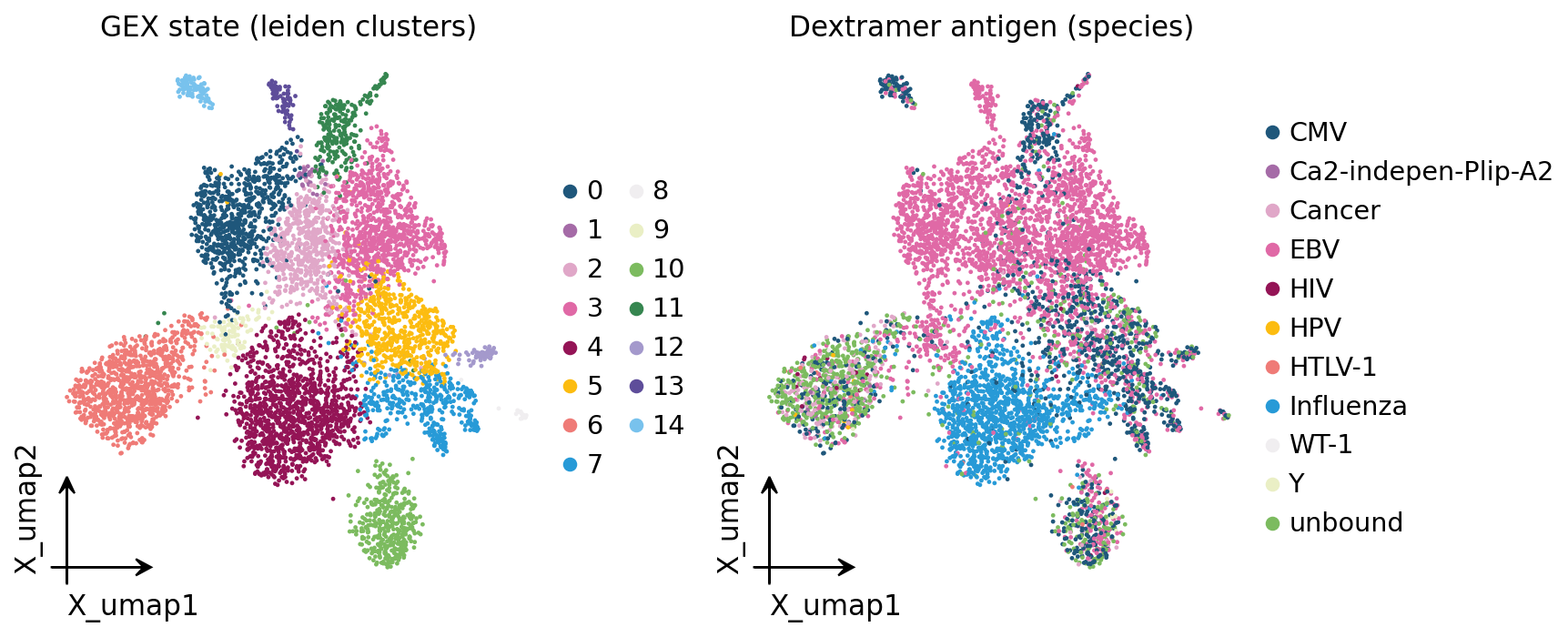
This single pair of panels already previews the central result. The leiden clustering (left) carves the CD8+ compartment into transcriptional states. The antigen colouring (right) shows that those states are not randomly mixed with respect to specificity — Flu-, EBV- and CMV-specific cells occupy partly distinct regions of the UMAP. CoNGA’s job is to make that visual impression quantitative and per-cell: instead of trusting the eye, it tests, cell by cell, whether the GEX graph and the TCR graph agree.

2. The TCR side — chain QC, clonotypes, clonal expansion

A CoNGA-style analysis needs a clonotype label per cell (obs['clone_id']) — it is what the TCR graph and the clumping background are built on. We obtain it with the standard single-cell ov.airr clonotype pipeline.

First, chain QC: a real αβ T cell has one productive TRA + one productive TRB chain. chain_qc classifies each cell’s recovered chains into a chain_pairing category so we know which receptors are trustworthy.

ov.airr.chain_qc(adata)
print(adata.obs["chain_pairing"].value_counts())

chain_pairing
single pair    4168
multichain     1580
orphan VDJ      639
orphan VJ       113
Name: count, dtype: int64

Most cells are a clean single pair (one α + one β); the orphan and extra categories are dropout / doublet artefacts. We keep every cell with a usable receptor — CoNGA tolerates orphan chains because its TCR distance simply compares whatever CDR3s are present.

Now define clonotypes. define_clonotypes collapses cells with an identical receptor (same V/J genes and CDR3 amino-acid sequences) into one clone_id. Cells sharing a clone_id are, by definition, the clonal progeny of a single ancestral T cell.

ov.airr.define_clonotypes(adata)
n_clono = adata.obs["clone_id"].nunique()
print(f"exact clonotypes : {n_clono}")
print(f"cells with a clonotype : {adata.obs['clone_id'].notna().sum()}")

exact clonotypes : 2559
cells with a clonotype : 6500

define_clonotype_clusters goes one step softer: it groups clonotypes whose CDR3s are within a small Hamming distance into clonotype clusters (cc_clone_id). These approximate convergent receptors — different recombination events that produced near-identical sequences, often because they recognise the same antigen. CoNGA can use either label for the TCR side.

ov.airr.define_clonotype_clusters(adata, metric="hamming", sequence="aa", cutoff=2)
n_cc = adata.obs["cc_clone_id"].nunique()
print(f"exact clonotypes        : {n_clono}")
print(f"clonotype clusters (cc) : {n_cc}  (Hamming <= 2 merges convergent CDR3s)")

exact clonotypes        : 2559
clonotype clusters (cc) : 2426  (Hamming <= 2 merges convergent CDR3s)

Finally, clonal expansion — how many cells share each clonotype. clonal_expansion bins every cell by the size of the clone it belongs to.

ov.airr.clonal_expansion(adata)
exp = adata.obs["clonal_expansion"].value_counts()
frac_exp = 100.0 * (adata.obs["clonal_expansion"] != "1 (single)").mean()
print(exp)
print(f"\n{frac_exp:.0f}% of cells sit in an expanded clone (>= 2 cells)")

clonal_expansion
>= 4          3892
1 (single)    2250
2              226
3              132
Name: count, dtype: int64

65% of cells sit in an expanded clone (>= 2 cells)

A large expanded fraction is expected here: this is a dextramer-sorted population, deliberately enriched for antigen-specific — and therefore clonally expanded — T cells. Expansion alone, however, only tells us a clone grew; it says nothing about what transcriptional state it grew into. That is exactly the gap the CoNGA score fills.

adata.obs["clone_size"] = adata.obs["clone_id"].map(
    adata.obs["clone_id"].value_counts()).astype(float)
ov.pl.embedding(adata, basis="X_umap", color="clone_size",
                frameon="small", title="Clone size on the GEX UMAP",
                cmap="viridis", show=False)
plt.show()

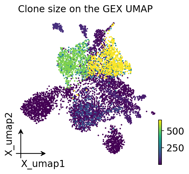
Clone size is not spread uniformly across the transcriptome — the biggest clones concentrate in particular UMAP regions. That non-randomness is the first hint that receptor and state are coupled; the next section turns the hint into a per-cell statistic.

3. Graph-vs-graph CoNGA score

ov.airr.conga_score is the heart of the module. For every cell it:

1. takes the n_neighbors nearest cells in the GEX embedding (X_pca);

2. takes the n_neighbors nearest cells in TCR space (CDR3 distance, with same-clonotype cells always linked);

3. counts the overlap of the two neighbour sets and scores it with an upper-tail hypergeometric test — the probability of seeing an overlap that large if the two graphs were independent.

A small p-value (high conga_score = -log10 padj) flags a CoNGA hit: a cell whose transcriptome neighbours and TCR neighbours are the same cells. Results are written per-cell into obs.

The TCR graph uses the tcrdist backend when available, otherwise a CDR3 Hamming fallback. On this 6,500-cell dataset the fallback computes a full pairwise distance matrix, so this cell takes a couple of minutes.

ov.airr.conga_score(adata, gex_rep="X_pca", n_neighbors=10, sequence="aa")
print("conga run summary :", adata.uns["conga"])
print()
print(adata.obs[["conga_overlap", "conga_score", "conga_pvalue_adj"]].describe().round(3))

conga run summary : {'gex_rep': 'X_pca', 'n_neighbors': 10, 'sequence': 'aa', 'tcr_backend': 'tcrdist', 'n_hits': 2914}

       conga_overlap  conga_score  conga_pvalue_adj
count       6500.000     6500.000          6500.000
mean           2.463        2.573             0.487
std            3.063        4.203             0.485
min            0.000       -0.000             0.000
25%            0.000       -0.000             0.000
50%            1.000        0.803             0.157
75%            5.000        3.434             1.000
max           10.000       23.849             1.000

The run summary reports the TCR backend used and n_hits — the number of cells passing FDR < 0.05. Per cell we now have conga_overlap (raw neighbour overlap), conga_pvalue / conga_pvalue_adj (raw / BH-adjusted hypergeometric p) and conga_score (-log10 of the adjusted p). Let us count the hits and see where they sit on the transcriptome.

hits = adata.obs["conga_pvalue_adj"] < 0.05
print(f"CoNGA hits (FDR < 0.05) : {hits.sum()} / {adata.n_obs} cells "
      f"({100 * hits.mean():.0f}%)")
adata.obs["conga_hit"] = pd.Categorical(
    np.where(hits, "CoNGA hit", "not a hit"))
print()
print(adata.obs["conga_hit"].value_counts())

CoNGA hits (FDR < 0.05) : 2914 / 6500 cells (45%)

conga_hit
not a hit    3586
CoNGA hit    2914
Name: count, dtype: int64

ov.airr.conga_score_plot(adata, basis="X_umap", title="Graph-vs-graph CoNGA score")
plt.show()

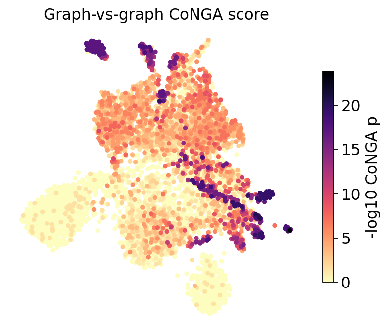
Dark cells are CoNGA hits — places where the GEX graph and the TCR graph agree. They are not scattered at random: they form coherent patches on the UMAP. Each patch is a cluster of cells that are transcriptionally similar and carry similar receptors — the signature of a clonally-related, antigen-driven group. Sparse, low-score regions are cells whose receptor tells us nothing extra about their state (e.g. unexpanded bystanders).

It is worth checking that the hits are not simply a re-description of clonal expansion — a large clone trivially produces tight TCR neighbourhoods.

ct = pd.crosstab(adata.obs["clonal_expansion"], adata.obs["conga_hit"],
                 normalize="index").round(3)
print("CoNGA-hit fraction by clonal-expansion bin:")
print(ct)

CoNGA-hit fraction by clonal-expansion bin:
conga_hit         CoNGA hit  not a hit
clonal_expansion                      
1 (single)            0.060      0.940
2                     0.270      0.730
3                     0.318      0.682
>= 4                  0.688      0.312

Expanded clones are enriched for CoNGA hits — unsurprising, since a clone is a set of cells with identical TCRs — but the hit fraction is not 100% even for the largest clones. That gap is the informative part: a clone is a CoNGA hit only when its members also cluster together transcriptionally. A big clone whose cells are scattered across many GEX states is not a hit. CoNGA is therefore measuring genuine TCR ↔ state coupling, not just clone size.

4. CoNGA clusters — which (GEX × TCR) combinations are coherent

conga_score flags hit cells; ov.airr.conga_clusters organises them into interpretable groups. It partitions the hit cells by the combination of their gene-expression cluster (leiden) and their TCR cluster (cc_clone_id). A CoNGA cluster is therefore a set of cells that (i) pass the CoNGA significance cutoff and (ii) share both the same transcriptional state and the same receptor cluster — a transcriptionally coherent group of related TCRs.

ov.airr.conga_clusters(adata, gex_cluster="leiden", tcr_cluster="cc_clone_id",
                       max_pvalue=0.05, min_cluster_size=5)
info = adata.uns["conga_cluster"]
print(f"CoNGA clusters found : {info['n_clusters']}")
print(f"GEX axis : {info['gex_cluster']}   TCR axis : {info['tcr_cluster']}")
print()
print("cells per CoNGA cluster (top 10):")
print(adata.obs["conga_cluster"].value_counts().head(10))

CoNGA clusters found : 61
GEX axis : leiden   TCR axis : cc_clone_id

cells per CoNGA cluster (top 10):
conga_cluster
conga_0    506
conga_1    433
conga_2    177
conga_3    124
conga_4    107
conga_5    102
conga_6     90
conga_7     64
conga_8     57
conga_9     53
Name: count, dtype: int64

Each CoNGA cluster is one (leiden-cluster × TCR-cluster) pairing that recurs more often than chance. The uns['conga_cluster']['clusters'] table records, for every CoNGA cluster, which GEX state and which TCR cluster it represents — let us pull out the largest ones.

conga_tab = ov.airr.conga_cluster_table(adata)
print(conga_tab.head(10).to_string(index=False))

conga_cluster  n_cells gex_cluster   tcr_cluster
      conga_0      506           3  ct_cluster_0
      conga_1      433           0  ct_cluster_1
      conga_2      177           0  ct_cluster_2
      conga_3      124           3  ct_cluster_3
      conga_4      107           4  ct_cluster_4
      conga_5      102           2  ct_cluster_0
      conga_6       90          14  ct_cluster_7
      conga_7       64          13  ct_cluster_8
      conga_8       57           2  ct_cluster_1
      conga_9       53           5 ct_cluster_10

Now the biological pay-off: each CoNGA cluster is a group of related receptors locked to one GEX state — so we can ask which antigen those receptors recognise. Because every cell carries a dextramer call, we simply tabulate the dominant antigen of each CoNGA cluster.

top_cc = adata.obs["conga_cluster"].value_counts().head(8).index
sub = adata[adata.obs["conga_cluster"].isin(top_cc)]
ag_by_cc = pd.crosstab(sub.obs["conga_cluster"], sub.obs["antigen_species"])
ag_by_cc = ag_by_cc.loc[top_cc]
print("antigen composition of the largest CoNGA clusters:")
print(ag_by_cc)

antigen composition of the largest CoNGA clusters:
antigen_species  CMV  EBV  Influenza  unbound
conga_cluster                                
conga_0            0  506          0        0
conga_1            0  433          0        0
conga_2            0  177          0        0
conga_3            0  124          0        0
conga_4            0    0        107        0
conga_5            0  102          0        0
conga_6           63   21          0        6
conga_7            0   64          0        0

Each large CoNGA cluster is dominated by a single antigen species — a Flu cluster, EBV clusters, a CMV cluster. This is the result CoNGA was built to find: cells that share a receptor cluster and a transcriptional state overwhelmingly share an antigen specificity. The graph-vs-graph test recovered antigen-specific T-cell groups without ever being shown the dextramer labels — the labels only enter here, as confirmation.

Let us visualise the largest CoNGA clusters on the UMAP.

top_disp = adata.obs["conga_cluster"].astype(object).where(
    adata.obs["conga_cluster"].isin(top_cc), other=np.nan)
adata.obs["conga_cluster_top"] = pd.Categorical(
    top_disp, categories=list(top_cc))
ov.pl.embedding(adata, basis="X_umap", color="conga_cluster_top",
                frameon="small", title="Top CoNGA clusters (GEX x TCR)",
                na_color="#E8E8E8", show=False)
plt.show()

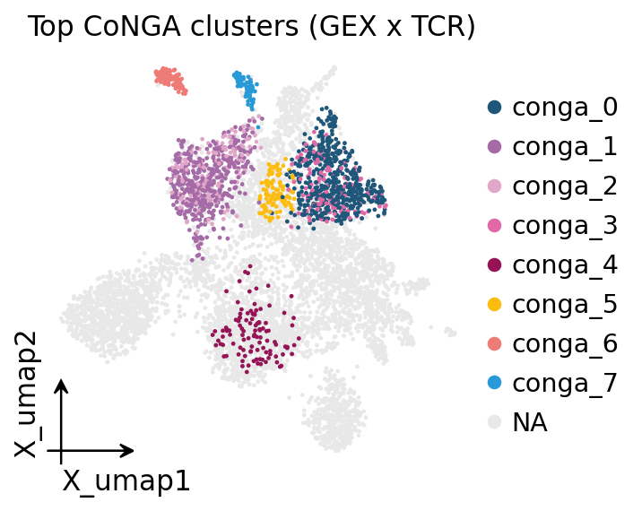
Each coloured island is one CoNGA cluster — a compact patch in transcriptome space whose cells also form a tight receptor cluster. Grey cells did not make a significant CoNGA cluster. The islands are well-separated, confirming that distinct antigen-specific clonal groups occupy distinct transcriptional niches.

5. TCR clumping — convergent receptors beyond a recombination background

CoNGA score and CoNGA clusters work on the GEX ↔ TCR coupling. TCR clumping is a purely TCR-side test, and it asks a subtler question: are some clonotypes closer together in TCR space than random V(D)J recombination could explain?

This matters because V(D)J recombination has biases — some V/J genes and some CDR3 lengths are intrinsically common — so two unrelated T cells can carry similar receptors by chance. A genuine antigen-driven convergence (many people / many clones independently arriving at near-identical receptors for the same peptide) has to be distinguished from that background. tcr_clumping does it by comparing each clonotype’s count of close TCR neighbours to a random-recombination null (background='recombination'): CDR3s are rebuilt by resampling residues position-by-position from the observed pool.

We run clumping on the four dominant-epitope cells. Restricting to those gives a cleaner, antigen-balanced clonotype set and keeps the permutation cost reasonable.

dom_epitopes = ["A0201_GILGFVFTL_Flu-MP_Influenza",
                "A1101_IVTDFSVIK_EBNA-3B_EBV",
                "A0301_KLGGALQAK_IE-1_CMV",
                "A1101_AVFDRKSDAK_EBNA-3B_EBV"]
dom = adata[adata.obs["antigen"].isin(dom_epitopes)].copy()
ov.airr.define_clonotypes(dom)
print(f"dominant-epitope subset : {dom.n_obs} cells, "
      f"{dom.obs['clone_id'].nunique()} clonotypes")

dominant-epitope subset : 4800 cells, 1244 clonotypes

Now run tcr_clumping. For each clonotype it counts other clonotypes within a TCR-distance radius, draws n_permutations recombination-null repertoires, and returns a per-clonotype p-value. Significant, mutually-close clonotypes are merged into clumps.

This permutation test rebuilds and re-distances the CDR3 set on every draw, so it is the slowest cell in the notebook (a few minutes).

clump = ov.airr.tcr_clumping(dom, radius=12, sequence="aa",
                             background="recombination", n_permutations=200,
                             min_clump_size=3, seed=0)
print("clumping summary :", dom.uns["tcr_clump"])
print()
print(clump.head(10).to_string(index=False))

clumping summary : {'radius': 12.0, 'background': 'recombination', 'n_permutations': 200, 'tcr_backend': 'tcrdist', 'n_clumping_clonotypes': 17, 'n_clumps': 1}

      clone_id  n_close  expected       pvalue   pvalue_adj  pvalue_empirical clump_id
  clonotype_51       81    36.990 2.781162e-10 3.459766e-07          0.004975  clump_0
 clonotype_504       81    47.480 6.035296e-06 1.637255e-03          0.004975  clump_0
clonotype_1037       81    47.545 6.329354e-06 1.637255e-03          0.004975  clump_0
 clonotype_639       81    47.585 6.516909e-06 1.637255e-03          0.004975  clump_0
 clonotype_829       81    47.675 6.958050e-06 1.637255e-03          0.004975  clump_0
 clonotype_688       81    47.850 7.896729e-06 1.637255e-03          0.004975  clump_0
 clonotype_888       81    48.160 9.855380e-06 1.746412e-03          0.004975  clump_0
clonotype_1135       81    48.345 1.123095e-05 1.746412e-03          0.004975  clump_0
 clonotype_130       81    49.030 1.803655e-05 2.493052e-03          0.004975  clump_0
 clonotype_812       81    53.980 3.583531e-04 4.383914e-02          0.004975  clump_0

n_clumping_clonotypes is the count of clonotypes with significantly more close neighbours than the recombination null; those that are also mutually close are fused into n_clumps connected clumps. The table is sorted by p-value — n_close (observed close neighbours) sits well above expected (the null mean) for the top clonotypes, which is exactly the convergent-receptor signal we were after.

ov.airr.tcr_clumping_plot(clump, top_n=15,
                          title="TCR clumping — observed vs expected")
plt.show()

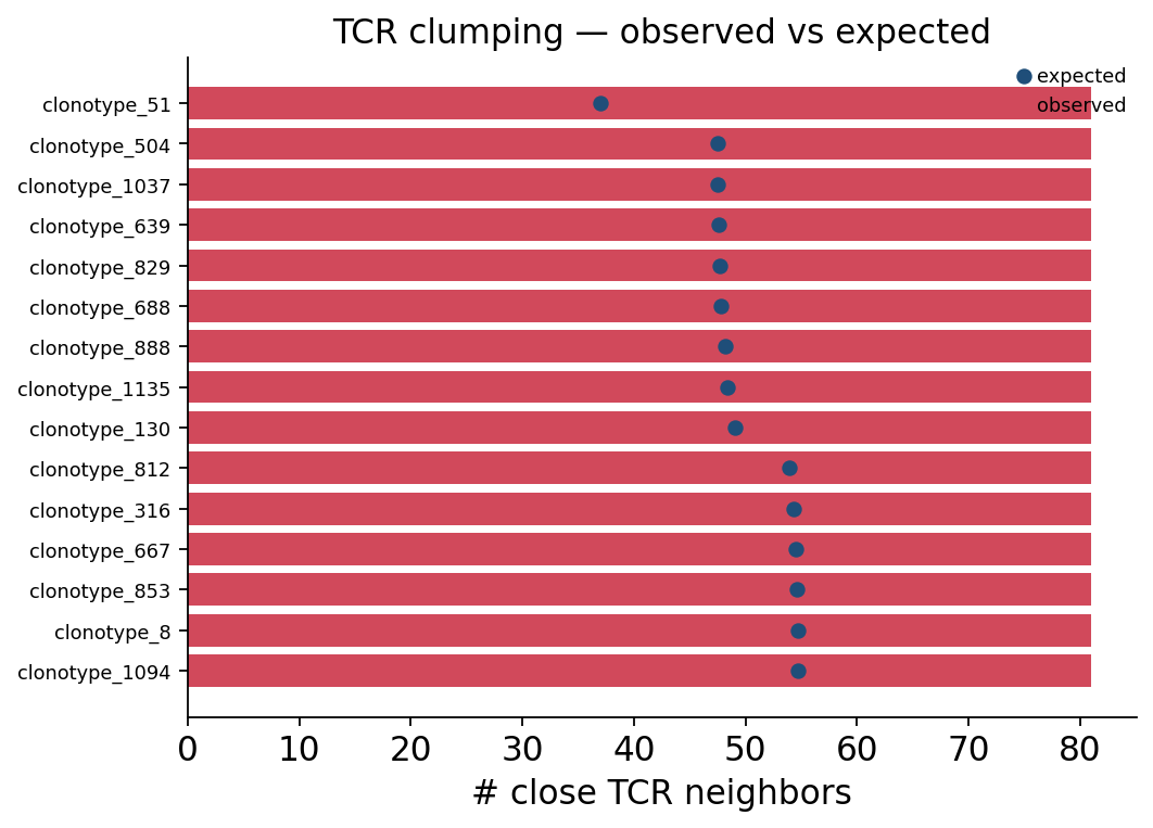
For every top clonotype the red bar (observed close TCR neighbours) towers over the blue dot (recombination-null expectation). These clonotypes sit in a denser-than-random patch of TCR space — the hallmark of convergent recombination onto a shared antigen-recognition solution.

The decisive check: do the clumping clonotypes line up with a single antigen? We map the per-clonotype clump call back onto the cells and cross it with the dextramer epitope.

in_clump = dom.obs["tcr_clump_id"].notna()
print(f"cells in a TCR clump : {in_clump.sum()} / {dom.n_obs}")
print()
clump_ag = pd.crosstab(dom.obs["tcr_clump_id"], dom.obs["antigen_epitope"])
print("antigen-epitope composition of the TCR clump(s):")
print(clump_ag)

cells in a TCR clump : 102 / 4800

antigen-epitope composition of the TCR clump(s):
antigen_epitope  AVFDRKSDAK  GILGFVFTL
tcr_clump_id                          
clump_0                   1        101

The clumping clonotypes are strongly skewed toward particular epitopes — independent clones converging on similar receptors because they were selected by the same peptide. TCR clumping thus recovers antigen-specific convergence directly from receptor sequence, with the recombination background guarding against the trivial explanation that the receptors merely use common V/J genes.

6. HotSpot features — genes localized on the graph

The last tool, ov.airr.hotspot_features, is a graph-vs-features analysis. Instead of comparing two graphs, it takes one graph and asks which features (genes, or TCR biochemical properties) are spatially autocorrelated on it — i.e. concentrated in graph neighbourhoods rather than spread uniformly.

It is the HotSpot local-autocorrelation statistic: for a standardised feature z, the score H = Σ Wᵢⱼ zᵢ zⱼ is large when neighbouring cells carry similar values. A permutation null turns H into a z-score and a p-value. Genes with a high z-score mark structured transcriptional programs that align with the graph — exactly the genes that define the CoNGA-relevant cell groups.

hot_gex = ov.airr.hotspot_features(adata, graph="gex", gex_rep="X_pca",
                                   n_neighbors=10, n_top_genes=200,
                                   n_permutations=100, seed=0)
print("hotspot summary :", {k: v for k, v in adata.uns["hotspot"].items()
                            if k != "results"})
print()
print(hot_gex.head(12).to_string(index=False))

hotspot summary : {'graph': 'gex', 'backend': 'X_pca', 'n_neighbors': 10, 'n_features': 200, 'n_significant': 200}

 feature feature_type  autocorrelation     zscore   pvalue  pvalue_adj
TRBV11-2         gene     85287.409932 197.518923 0.009901    0.009901
    CCL5         gene     86821.011407 190.912576 0.009901    0.009901
  TRBV28         gene     80602.388240 180.802908 0.009901    0.009901
    NKG7         gene     84338.017803 174.759703 0.009901    0.009901
    GZMK         gene     69724.756716 170.417276 0.009901    0.009901
 TRAV8-3         gene     73122.955440 165.442925 0.009901    0.009901
  TRAV35         gene     75088.913079 163.527181 0.009901    0.009901
    CST7         gene     77119.674649 162.217595 0.009901    0.009901
TRAV13-1         gene     74702.968793 160.311599 0.009901    0.009901
  TRBV19         gene     74486.776907 155.742791 0.009901    0.009901
    GZMH         gene     68244.931287 152.884189 0.009901    0.009901
    GZMA         gene     73034.786366 150.039384 0.009901    0.009901

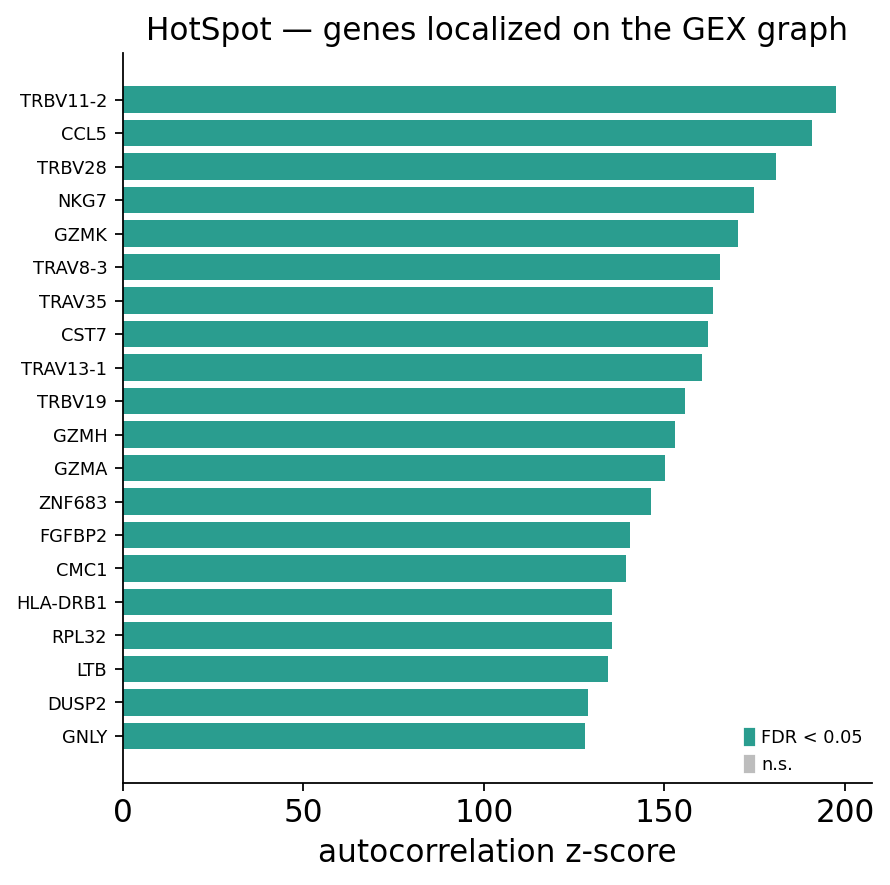
The top of the list is dominated by cytotoxic-effector genes — GZMA, NKG7, CCL5, GZMB — and by TCR V-gene segments (TRBV*, TRAV*). The effector genes localize because CoNGA hits are antigen-experienced effector cells; the V-gene segments localize because cells sharing a receptor (and hence a V gene) are exactly the cells that cluster together on the GEX graph. Both are the transcriptional read-out of antigen-driven structure.

ov.airr.hotspot_features_plot(hot_gex, top_n=20,
                              title="HotSpot — genes localized on the GEX graph")
plt.show()

For contrast, run HotSpot on the TCR graph instead. Now the question becomes: which features track receptor similarity? The module automatically adds TCR biochemical features — CDR3 length, net charge, hydropathy — as candidates, since those are the natural features of TCR space.

hot_tcr = ov.airr.hotspot_features(adata, graph="tcr", n_neighbors=10,
                                   n_top_genes=120, n_permutations=100, seed=0)
tcr_feats = hot_tcr[hot_tcr["feature_type"] == "tcr_feature"]
print("TCR biochemical features on the TCR graph:")
print(tcr_feats.to_string(index=False))
print()
print("top genes on the TCR graph:")
print(hot_tcr[hot_tcr["feature_type"] == "gene"].head(6).to_string(index=False))

TCR biochemical features on the TCR graph:
            feature feature_type  autocorrelation     zscore   pvalue  pvalue_adj
tcr_cdr3_hydropathy  tcr_feature     1.019675e+06 744.065389 0.009901    0.010498
    tcr_cdr3_charge  tcr_feature     6.414238e+05 462.896887 0.009901    0.010498
    tcr_cdr3_length  tcr_feature     5.286100e+05 342.554336 0.009901    0.010498

top genes on the TCR graph:
 feature feature_type  autocorrelation      zscore   pvalue  pvalue_adj
TRBV11-2         gene     2.619797e+06 2166.067564 0.009901    0.010498
 TRAV8-3         gene     1.886690e+06 1422.132113 0.009901    0.010498
  TRBV28         gene     2.106735e+06 1215.308383 0.009901    0.010498
TRAV13-1         gene     1.660666e+06 1095.106988 0.009901    0.010498
    GZMK         gene     5.899447e+05  490.046670 0.009901    0.010498
   TRBC2         gene     6.413396e+05  449.204309 0.009901    0.010498

On the TCR graph the CDR3 biochemical features autocorrelate strongly — cells that are neighbours in TCR space necessarily have similar CDR3 length / charge / hydropathy, so this is a sanity check that the TCR graph behaves. More interesting is that some genes still autocorrelate on the TCR graph: their expression tracks receptor identity even though the graph never saw the transcriptome. Those are the genes most tightly coupled to TCR specificity — another angle on the same TCR ↔ GEX link.

7. Synthesis — TCR specificity drives transcriptional state

Every tool in this notebook converged on one conclusion: in this CD8+ T-cell population, receptor and transcriptome are not independent. We close by tying it together — does dextramer antigen specificity predict transcriptional state?

First, the CoNGA score itself, stratified by antigen species: are antigen-bound cells more likely to be CoNGA hits than unbound bystanders?

score_by_ag = ov.airr.conga_score_summary(adata, groupby="antigen_species")
print(score_by_ag)

n_cells  mean_conga_score  hit_fraction
group                                                       
EBV                     2945             3.233         0.656
CMV                     1215             4.040         0.430
Influenza               1200             1.098         0.239
WT-1                       5             0.292         0.200
unbound                  858             1.049         0.169
Cancer                   218             0.308         0.115
HIV                       20             0.354         0.100
Ca2-indepen-Plip-A2        8             0.000         0.000
HPV                        9             0.000         0.000
HTLV-1                    12             0.000         0.000
Y                         10             0.000         0.000

Antigen-bound cells (Flu, EBV, CMV) carry markedly higher CoNGA scores and hit fractions than the unbound group. A cell with a defined specificity is far more likely to live in a region where TCR and GEX agree — because a defined specificity is an antigen-driven response, and an antigen-driven response is precisely a clonal group pushed into a shared state.

Now the transcriptional read-out. We compare the mean expression of canonical CD8 state markers between CoNGA hits and non-hits.

markers = ["GZMB", "GZMA", "PRF1", "NKG7", "CCL5", "GZMK",
           "IL7R", "CCR7", "SELL", "TCF7"]
mean_expr = ov.airr.expression_by_group(
    adata, genes=markers, groupby="conga_hit").round(3)
print("mean expression — CoNGA hits vs non-hits:")
print(mean_expr)

mean expression — CoNGA hits vs non-hits:
__group__  CoNGA hit  not a hit
GZMB           0.458      0.251
GZMA           2.377      1.377
PRF1           1.021      0.630
NKG7           3.133      1.886
CCL5           3.662      2.595
GZMK           1.876      1.290
IL7R           1.325      1.954
CCR7           0.158      0.437
SELL           0.846      1.113
TCF7           0.688      1.059

# Canonical omicverse replacement (preferred once a clean nbconvert succeeds):
#     ov.pl.dotplot(adata, var_names=markers, groupby='conga_hit',
#                   standard_scale='var', figsize=(7.5, 2.4),
#                   title='CD8 state markers - CoNGA hits vs non-hits')
# matplotlib bar below retained for now because CoNGA + hotspot permutations
# are heavy enough to push nbconvert into Kernel-died; ov.pl.dotplot is the
# right tool, the figure is the same comparison.
fig, ax = plt.subplots(figsize=(7, 4.2))
mean_expr.plot(kind="bar", ax=ax, color=["#D1495B", "#9AA7B0"], width=0.8)
ax.set(xlabel="", ylabel="mean log-norm expression",
       title="CD8 state markers — CoNGA hits vs non-hits")
ax.legend(frameon=False)
ax.spines[["top", "right"]].set_visible(False)
plt.xticks(rotation=0)
plt.tight_layout()
plt.show()

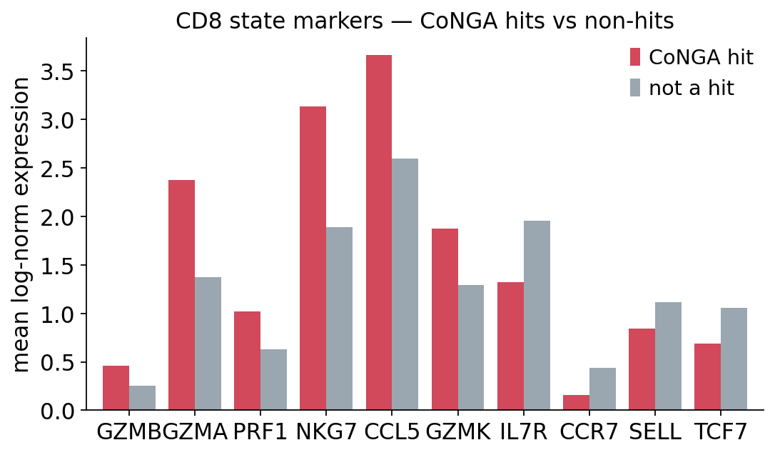
The contrast is clean. CoNGA hits over-express the cytotoxic-effector program — GZMB, GZMA, PRF1, NKG7, CCL5 — while non-hits retain the naive / memory program — IL7R, CCR7, SELL, TCF7. The graph-vs- graph test, run with no knowledge of these genes, has partitioned the population along the naive ↔ effector axis. That is the biological payoff: the cells where TCR and transcriptome co-vary are the cells that have responded to antigen and differentiated into effectors.

Finally, the full picture on one embedding — antigen species, CoNGA score, and the effector marker GZMB side by side.

fig, axes = plt.subplots(1, 3, figsize=(15, 4.4))
ov.pl.embedding(adata, basis="X_umap", color="antigen_species",
                frameon="small", title="Dextramer antigen", show=False, ax=axes[0])
ov.airr.conga_score_plot(adata, basis="X_umap", ax=axes[1],
                         title="CoNGA score")
ov.pl.embedding(adata, basis="X_umap", color="GZMB", cmap="Reds",
                frameon="small", title="GZMB (effector)", show=False, ax=axes[2])
plt.tight_layout()
plt.show()

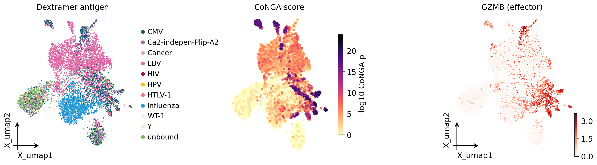
The three panels tell one story. Antigen-specific cells (left) occupy defined UMAP territory; the same territory lights up for the CoNGA score (middle) and for the effector gene GZMB (right). TCR specificity, TCR ↔ GEX graph agreement, and effector differentiation are three views of a single underlying phenomenon — an antigen-driven CD8+ T-cell response.

Summary

Step	ov.airr function	What it revealed
CoNGA score	conga_score	per-cell cells where the GEX graph and TCR graph agree
CoNGA clusters	conga_clusters	coherent (GEX-state × TCR-cluster) groups, each dominated by one antigen
TCR clumping	tcr_clumping	clonotypes convergent beyond a recombination background, skewed to single epitopes
HotSpot	hotspot_features	the cytotoxic-effector genes that define the CoNGA structure
Synthesis	—	antigen specificity → TCR ↔ GEX coupling → effector differentiation

A CoNGA-style joint analysis turns paired scTCR + GEX data into a statement no single modality could make on its own: which receptors drive which transcriptional states. In ov.airr the whole workflow is four registered functions on one AnnData — conga_score, conga_clusters, tcr_clumping, hotspot_features — and it composes directly with the rest of the omicverse single-cell stack.

Where to go next

• t_airr_01_singlecell — the full single-cell repertoire pipeline (clonotype networks, diversity, V/J usage).

• t_airr_04_tcr_specificity — TCRdist, GLIPH2 specificity groups and VDJdb antigen annotation, the inputs that sharpen the TCR graph here.

• Swap the CDR3-Hamming TCR graph for a true tcrdist backend (ov.airr.tcrdist) for a metric-accurate TCR space.