scATAC-seq preprocessing and quality control

omicverse.epi (ov.epi) brings epigenomics into OmicVerse by wrapping the epione toolkit. Every ov.epi function imports epione internally and delegates, so the familiar pp / tl / pl layout you know from the rest of OmicVerse now also covers single-cell ATAC-seq, bulk ATAC/ChIP, footprinting, chromVAR motif activity, peak-to-gene linkage and Hi-C.

This first tutorial walks the upstream half of a single-cell ATAC-seq analysis — turning a 10x fragments.tsv.gz into a quality-controlled cell × tile matrix ready for embedding:

1. ingest a fragments file (ov.epi.pp.import_fragments)

2. compute per-cell QC metrics — TSS enrichment, fragment-size periodicity, nucleosome signal

3. filter low-quality cells (ov.epi.pp.qc)

4. build a 500 bp genome-tile count matrix and select features

5. a first iterative-LSI embedding to sanity-check the result

We use the public 10x PBMC 500-cell scATAC dataset (GRCh38), which ov.epi.datasets downloads on demand — so the whole notebook is self-contained and runs on a laptop CPU.

import warnings
warnings.filterwarnings('ignore')

import numpy as np
import matplotlib.pyplot as plt

import omicverse as ov

# Confirm the epione backend is available and apply the publication plot style.
ov.epi.check_epione()
ov.epi.pl.plot_set()
print('omicverse', ov.__version__)

epione is available (version 0.0.1rc1); ov.epi is ready.
└─ 🔬 Starting plot initialization...
  ├─ Apply Scanpy/matplotlib settings
  ├─ Custom font setup
  ├─ Suppress warnings
  ├─ 
___________      .__                      
\_   _____/_____ |__| ____   ____   ____  
 |    __)_\____ \|  |/  _ \ /    \_/ __ \ 
 |        \  |_> >  (  <_> )   |  \  ___/ 
/_______  /   __/|__|\____/|___|  /\___  >
        \/|__|                  \/     \/ 

  ├─ 🔖 Version: 0.0.1rc1   📚 Tutorials: https://epione.readthedocs.io/
└─ ✅ plot_set complete.

omicverse 2.2.1rc1

1 · Load fragments

ov.epi.datasets.atac_pbmc500_fragments() fetches (and caches) the bgzipped, tabix-indexed 10x PBMC-500 fragments file. ov.epi.pp.import_fragments scans it into an AnnData carrying per-cell QC counts. We pass file= so the object is written out-of-memory (anndataoom-backed) — this is what lets the genome-wide tile matrix be added later without blowing up RAM.

The chromosome sizes / gene annotation come from ov.epi.data.hg38, a reference Genome that lazily downloads the GRCh38 FASTA + Gencode annotation via pooch on first use.

import os

frag = ov.epi.datasets.atac_pbmc500_fragments()
print('fragments file:', frag)

genome = ov.epi.data.hg38

work = os.path.join(os.getcwd(), 'data_epi')
os.makedirs(work, exist_ok=True)
h5 = os.path.join(work, 'pbmc500.h5ad')
if os.path.exists(h5):
    os.remove(h5)

adata = ov.epi.pp.import_fragments(
    str(frag),
    chrom_sizes=genome,
    file=h5,
    min_num_fragments=500,
)
adata

fragments file: /tmp/snapatac2/atac_pbmc_500.tsv.gz
└─ scanning /tmp/snapatac2/atac_pbmc_500.tsv.gz
└─ imported 646 cells  (9,899,673 unique fragments)

AnnDataOOM646obs×0varsRust · out-of-memory · backed

csr_matrix float32 · 0.0% · ~0.0 MB/chunk · 0 MB disk · pbmc500.h5ad

›obs3n_fragment · frac_dup · frac_mito

name	dtype	preview
n_fragment	int64	8964, 14968, 28335, … (639)
frac_dup	float64	0.6372172083046663, 0.6288986958893241, 0.7626347666557765, … (645)
frac_mito	float64	0.0

›empty–var · obsm · varm · obsp · varp · layers · raw

2 · Per-cell quality-control metrics

Three complementary QC signals tell us which barcodes are real, high-quality cells:

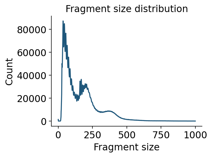
• TSS enrichment (tsse) — accessibility pile-up at transcription start sites vs. flanking background. High-quality ATAC sits well above 2–4.

• Fragment-size distribution — open chromatin shows a clean nucleosome ladder (a sub-100 bp nucleosome-free peak, then mono-/di-nucleosome shoulders at ~200/400 bp).

• Nucleosome signal — ratio of mono-nucleosome to nucleosome-free fragments per cell.

The TSS step needs gene coordinates, which we read from the bundled hg38 annotation.

genes = ov.epi.io.get_gene_annotation(genome)
print('gene annotation rows:', len(genes))

ov.epi.pp.tsse(adata, genes)
ov.epi.pp.frag_size_distr(adata)
ov.epi.pp.nucleosome_signal(adata)

# obs is a lazy on-disk element on the backed object; pull it into pandas for inspection.
obs = ov.epi.utils.obs_to_pandas(adata)
obs[['n_fragment', 'tsse', 'nucleosome_signal']].head()

gene annotation rows: 19978
└─ Computing TSS enrichment score for adata...
└─ Computing TSS enrichment score for adata...
└─ Added TSS enrichment score to adata.obs['tss_score']
└─ Created TSS enrichment score
  └─ Added TSS enrichment score to tss_pileup.obs['tss_score']
  └─ Returned TSS enrichment score
  └─ Added TSS enrichment score to adata.obs['tsse']
└─ Computing fragment size distribution for adata...
└─ Added fragment size distribution to adata.uns['frag_size_distr']
└─ Computing nucleosome signal for adata...
└─ Added a "nucleosome_signal" column to the .obs slot of the AnnData object
└─ Created nucleosome signal
  └─ Added nucleosome signal to adata.obs['nucleosome_signal']

	n_fragment	tsse	nucleosome_signal
obs_names
AAACTGCAGACTCGGA-1	8964	27.805281	0.572474
AAAGATGCACCTATTT-1	14968	25.742574	0.491104
AAAGATGCAGATACAA-1	28335	39.995482	0.456936
AAAGGGCTCGCTCTAC-1	28541	25.804671	0.719165
AAATGAGAGTCCCGCA-1	7749	37.316490	0.425304

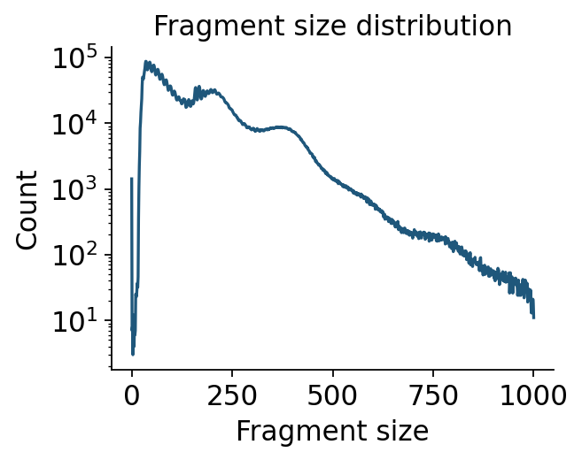
Fragment-size periodicity

The nucleosome ladder is one of the cleanest ATAC QC signatures. ov.epi.pl.frag_size_distr plots the distribution computed above; the log-y view makes the di-nucleosome shoulder visible.

ov.epi.pl.frag_size_distr(adata, figsize=(4, 3))
plt.show()
ov.epi.pl.frag_size_distr(adata, figsize=(4, 3), log_y=True)
plt.show()

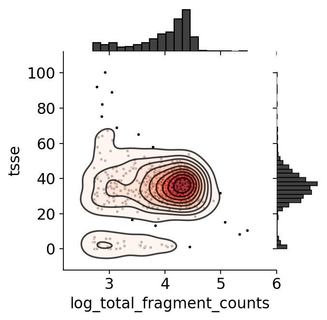
Joint QC scatter

A log-fragment-count vs. TSS-enrichment scatter is the classic ATAC QC view: good cells sit in the upper-right (high coverage and high TSS enrichment).

# Joint QC scatter via epione's ATAC-native plotter (log-fragments vs TSSe).
obs['log_total_fragment_counts'] = np.log10(obs['n_fragment'])
ov.epi.pl.plot_joint(adata, x_col='log_total_fragment_counts', y_col='tsse',
                     kde_kwargs={'cut': 3})
plt.show()

3 · Filter low-quality cells

ov.epi.pp.qc applies thresholds on all metrics at once. We keep cells with 1000–100000 fragments, TSS enrichment ≥ 2 and nucleosome signal ≤ 4.

adata = ov.epi.pp.qc(adata, tresh={
    'fragment_counts_min': 1000,
    'fragment_counts_max': 100000,
    'TSS_score_min':       2.0,
    'TSS_score_max':       100.0,
    'Nucleosome_singal_max': 4.0,
})
print('cells passing QC:', adata.n_obs)
adata

└─ Performing QC...
  └─ Filtering cells based on fragment counts...
  └─ Filtering cells based on nucleosome signal...
  └─ Filtered 78 cells
cells passing QC: 568

AnnDataOOM568obs×0varsRust · lazy · backed

csr_matrix float32 · 0.0% · ~0.0 MB/chunk · 0 MB disk · pbmc500.h5ad

›obs8n_fragment · frac_dup · frac_mito · tss_score · tsse · nucleosome_signal +2

name	dtype	preview
n_fragment	int64	8964, 14968, 28335, … (565)
frac_dup	float64	0.6372172083046663, 0.6288986958893241, 0.7626347666557765, … (568)
frac_mito	float64	0.0
tss_score	float64	27.805280528052805, 25.742574257425744, 39.995482437977635, … (560)
tsse	float64	27.805280528052805, 25.742574257425744, 39.995482437977635, … (560)
nucleosome_signal	float64	0.5724738675958189, 0.4911038836808877, 0.4569364161849711, … (568)
log_total_fragment_counts	float64	3.9525018478630236, 4.175163774491954, 4.452323216977515, … (565)
selected	bool	True

›empty–var · obsm · varm · obsp · varp · layers · raw

›chain2transform pipeline

[0]backedBackedArray646 × 0 · Rust (anndata-rs)

[1]subset_SubsetBackedArray568 × 0 · obs: 568

4 · Tile matrix and feature selection

For unbiased clustering we bin the genome into 500 bp tiles and count per-cell insertions (add_tile_matrix), then keep the most-accessible features (select_features).

ov.epi.pp.add_tile_matrix(adata, bin_size=500)
ov.epi.pp.select_features(adata, n_features=250000)
print('tile matrix:', adata.shape)
print('features selected:', int(np.asarray(adata.var['selected']).sum()))

└─ building tile matrix: 568 cells × 6,176,584 tiles (500 bp bins, strategy=paired-insertion)
└─ tile matrix nnz=9,644,952
└─ Selected 250,000 features.
tile matrix: (568, 6176584)
features selected: 250000

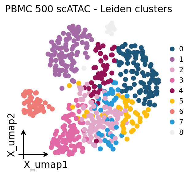
5 · A first embedding

ArchR-style iterative LSI (ov.epi.tl.iterative_lsi) is the standard scATAC dimensionality reduction: binarize → TF-IDF → SVD, iterated with intermediate clustering to focus on variable features. We then build a neighbor graph, cluster and embed with UMAP — the same pp/tl verbs as the RNA workflow.

ov.epi.tl.iterative_lsi(adata, n_components=20, iterations=2)
ov.epi.pp.neighbors(adata, use_rep='X_iterative_lsi')
ov.epi.tl.clusters(adata, method='leiden', use_rep='X_iterative_lsi', key_added='clusters')
ov.epi.tl.umap(adata)
print('embeddings:', list(adata.obsm.keys()))

└─ [iterative_lsi] Initial feature set: 500,000 / 6,176,584
  └─ [iterative_lsi] Iter 1/2 | fit on 568 cells x 500,000 features
computing neighbors
finished: added to `.uns['neighbors']`
    `.obsp['distances']`, distances for each pair of neighbors
    `.obsp['connectivities']`, weighted adjacency matrix (0:00:07)
running Leiden clustering
finished: found 7 clusters and added
    'leiden', the cluster labels (adata.obs, categorical) (0:00:00)
└─ [iterative_lsi]   -> 7 clusters; selected 25,000 variable features for next round
  └─ [iterative_lsi] Iter 2/2 | fit on 568 cells x 25,000 features
└─ [iterative_lsi] Done. Stored embedding (568 x 19) in adata.obsm['X_iterative_lsi']
Computing neighbors with n_neighbors=15
Finished computing neighbors
    Added to .uns['neighbors']
    .obsp['distances'], distances for each pair of neighbors
    .obsp['connectivities'], weighted adjacency matrix
Running Leiden clustering with leidenalg...
    Finished: found 9 clusters
    Added 'clusters' to adata.obs (categorical)
Computing UMAP embedding...
Finished computing UMAP
    Added:
        'X_umap', UMAP coordinates (adata.obsm)
        'umap', UMAP parameters (adata.uns)
embeddings: ['X_iterative_lsi', 'X_umap']

# Plot the embedding with omicverse's standard plotter. The QC AnnData is
# anndataoom-backed, so we wrap the UMAP + cluster labels in a light in-memory
# AnnData for ov.pl.embedding.
import anndata as ad
obs = ov.epi.utils.obs_to_pandas(adata)
pa = ad.AnnData(np.zeros((adata.n_obs, 1), dtype='float32'))
pa.obs_names = list(adata.obs_names)
pa.obs['clusters'] = obs['clusters'].astype('category').values
pa.obsm['X_umap'] = np.asarray(adata.obsm['X_umap'])
ov.pl.embedding(pa, basis='X_umap', color='clusters', frameon='small',
                title='PBMC 500 scATAC - Leiden clusters', show=False)
plt.show()

Summary

Starting from a raw 10x fragments file we produced a QC-filtered, embedded scATAC dataset using only ov.epi:

stage	function
ingest fragments	ov.epi.pp.import_fragments
TSS enrichment	ov.epi.pp.tsse
fragment size / nucleosome	ov.epi.pp.frag_size_distr, ov.epi.pp.nucleosome_signal
QC filter	ov.epi.pp.qc
tile matrix / features	ov.epi.pp.add_tile_matrix, ov.epi.pp.select_features
embed / cluster	ov.epi.tl.iterative_lsi, ov.epi.pp.neighbors, ov.epi.tl.clusters, ov.epi.tl.umap

The next tutorial picks up from a larger annotated PBMC dataset to cover clustering, cell-type annotation and gene-activity scores.