Bulk Hi-C — contact maps, compartments and TADs#
Hi-C measures the 3D folding of the genome: how often any two loci contact each other. ov.epi
wraps epione’s Hi-C analysis (ov.epi.bulk.hic.*, built on cooler + cooltools) so the standard
analyses — contact matrices, the distance-decay curve P(s), A/B compartments, and topologically
associating domains (TADs) — are a few calls.
Data. This tutorial uses a balanced Drosophila S2 .cool (10 kb bins) from the HiCExplorer /
Galaxy Hi-C training set. Point the COOL path below at your own balanced .cool /
.mcool::/resolutions/N; the upstream FASTQ→pairs→cool steps live in ov.epi.upstream
(pairs_from_bam, pairs_to_cool). Everything downstream is generic to any balanced cooler.
import warnings
warnings.filterwarnings('ignore')

import pathlib
import numpy as np
import pandas as pd
import matplotlib.pyplot as plt
import cooler

import omicverse as ov
ov.epi.pl.plot_set()
print('omicverse', ov.__version__)

DATA = pathlib.Path('/scratch/users/steorra/data/drosophila-hic')
COOL = str(DATA / 'drosophila.cool')
FASTA = str(DATA / 'dm3_genome.fasta')   # used only to GC-phase the compartments

hic = ov.epi.bulk.hic
clr = cooler.Cooler(COOL)
print('resolution:', clr.binsize, 'bp | bins:', clr.info['nbins'], '| chroms:', clr.chromnames[:6])
└─ 🔬 Starting plot initialization...
  ├─ Apply Scanpy/matplotlib settings
  ├─ Custom font setup
  ├─ Suppress warnings
  ├─
___________      .__
\_   _____/_____ |__| ____   ____   ____
 |    __)_\____ \|  |/  _ \ /    \_/ __ \
 |        \  |_> >  (  <_> )   |  \  ___/
/_______  /   __/|__|\____/|___|  /\___  >
        \/|__|                  \/     \/

  ├─ 🔖 Version: 0.0.1rc1   📚 Tutorials: https://epione.readthedocs.io/
└─ ✅ plot_set complete.

omicverse 2.2.1rc1
resolution: 10000 bp | bins: 16880 | chroms: ['chr2L', 'chr2LHet', 'chr2R', 'chr2RHet', 'chr3L', 'chr3LHet']
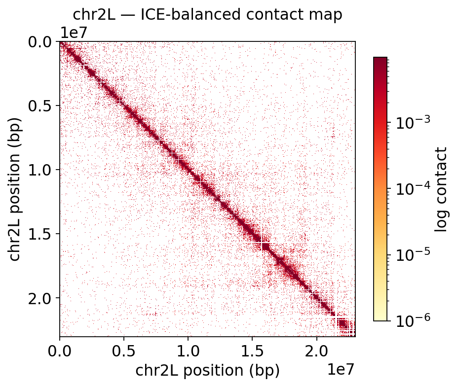
1 · Contact matrices#
ov.epi.bulk.hic.plot_contact_matrix reads the cooler directly and renders an ICE-balanced,
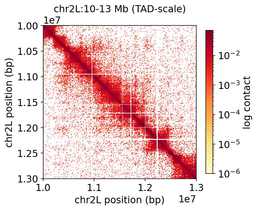
log-scaled heatmap for any region — a whole chromosome arm, then a 3 Mb zoom where TAD structure
appears as on-diagonal blocks.
fig, ax, _ = hic.plot_contact_matrix(
    COOL, region='chr2L', balance=True, log=True,
    figsize=(6, 5.5), title='chr2L — ICE-balanced contact map')
plt.show()
fig, ax, _ = hic.plot_contact_matrix(
    COOL, region='chr2L:10_000_000-13_000_000', balance=True, log=True,
    figsize=(5, 4.8), title='chr2L:10-13 Mb (TAD-scale)')
plt.show()
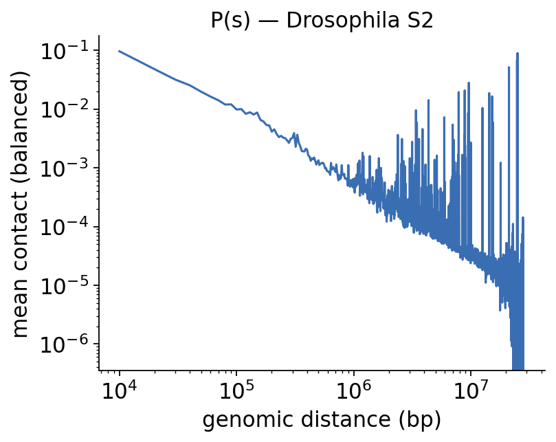
2 · Distance decay P(s)#
Contact frequency falls off with genomic distance — the P(s) curve. Its shape is a global summary of chromatin folding and a key QC for any Hi-C library.
fig, ax, decay = hic.plot_decay_curve(COOL, balance=True, figsize=(5.2, 4),
                                      title='P(s) — Drosophila S2')
plt.show()
decay.head()
| chrom | offset_bin | distance_bp | mean_contact | n_pairs | |
|---|---|---|---|---|---|
| 0 | chr2L | 0 | 0 | 0.263320 | 2222 |
| 1 | chr2L | 1 | 10000 | 0.120140 | 2177 |
| 2 | chr2L | 2 | 20000 | 0.056927 | 2167 |
| 3 | chr2L | 3 | 30000 | 0.037639 | 2168 |
| 4 | chr2L | 4 | 40000 | 0.028203 | 2164 |
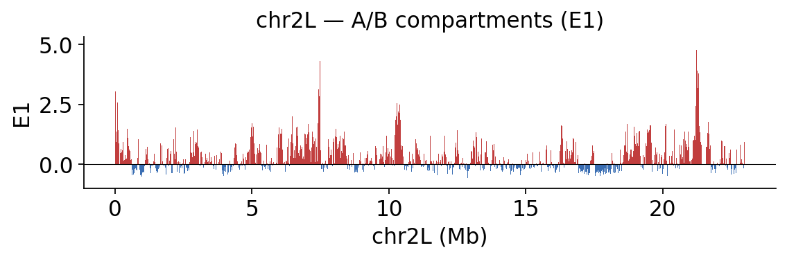
3 · A/B compartments#
At the megabase scale chromatin separates into an active A and inactive B compartment.
ov.epi.bulk.hic.compartments computes the eigenvector decomposition of the observed/expected
matrix; GC content (from the FASTA) is used to sign E1 so that positive E1 = A.
comp = hic.compartments(COOL, chromosomes=['chr2L', 'chr2R', 'chr3L', 'chr3R'],
                        fasta_path=FASTA)
print(comp[['chrom', 'start', 'end', 'E1']].head())

fig, ax = hic.plot_compartments(comp, chromosome='chr2L', track_column='E1',
                                title='chr2L — A/B compartments (E1)')
plt.show()
chrom  start    end        E1
0  chr2L      0  10000       NaN
1  chr2L  10000  20000  3.049649
2  chr2L  20000  30000  1.300753
3  chr2L  30000  40000  0.920896
4  chr2L  40000  50000  0.490555
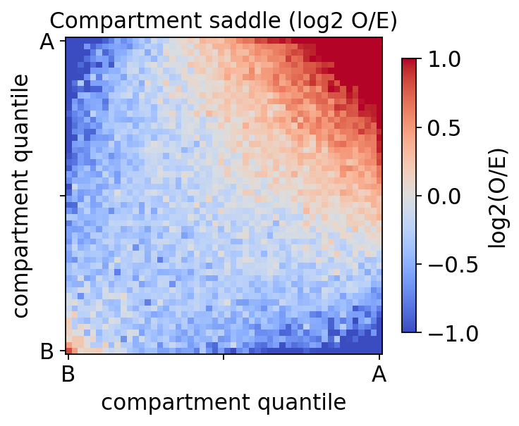
Saddle plot#
A saddle plot summarises compartmentalisation strength: binning the O/E matrix by compartment eigenvalue, A–A and B–B contacts (corners) are enriched over A–B (off-diagonal).
saddle = hic.saddle(COOL, comp, chromosomes=['chr2L', 'chr2R', 'chr3L', 'chr3R'])
mat, edges = saddle[0], saddle[1]   # (saddle matrix, bin edges, count matrix)
fig, ax, _ = hic.plot_saddle(mat, edges=edges, title='Compartment saddle (log2 O/E)')
plt.show()
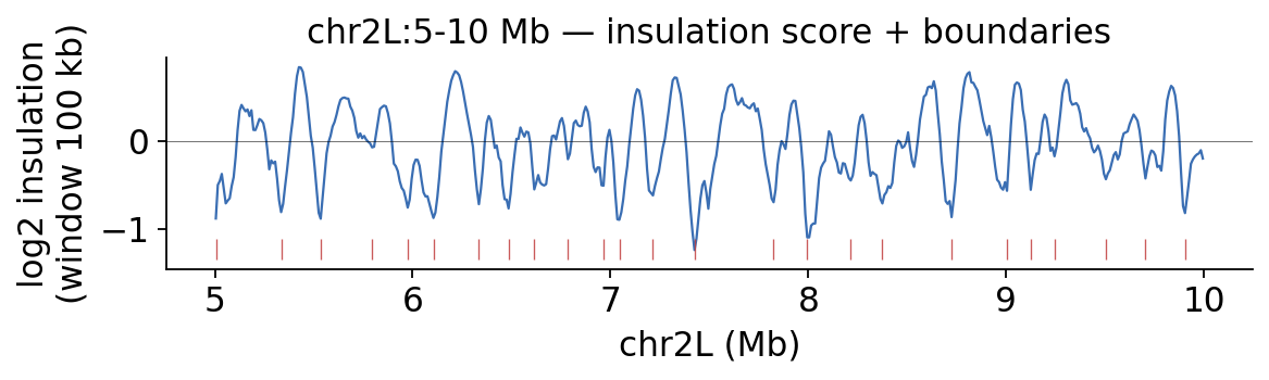
4 · Insulation and TAD boundaries#
At finer scale the genome folds into TADs. The diamond insulation score
(ov.epi.bulk.hic.insulation) dips at domain boundaries; tad_boundaries calls them.
ins = hic.insulation(COOL, window_bp=100_000, chromosomes=['chr2L'], ignore_diags=2)
bounds = hic.tad_boundaries(ins)
print('insulation bins:', len(ins), '| TAD boundaries called:', len(bounds))

fig, ax = hic.plot_insulation(
    ins, chromosome='chr2L', region_start=5_000_000, region_end=10_000_000,
    title='chr2L:5-10 Mb — insulation score + boundaries')
plt.show()
insulation bins: 2302 | TAD boundaries called: 96
Summary#
stage |
function |
|---|---|
contact matrix |
|
distance decay P(s) |
|
A/B compartments |
|
TAD insulation |
|
All operate directly on a cooler file, so the same calls work on any organism and resolution.
The companion tutorial covers single-cell Hi-C.