Single-cell metabolic landscape of a head & neck tumour#
scRNA-seq measures mRNA, not metabolites — but the transcriptome
carries a strong, recoverable signal of a cell’s metabolic state.
This tutorial runs a complete metabolic analysis of a real tumour,
reproducing the landmark study Xiao, Dai & Locasale, Nat Commun
2019 — “Metabolic landscape of the tumor microenvironment at single
cell resolution” on its head & neck cancer cohort, with
ov.single.Metabolism.
Part.1 The question and the approach#
A tumour is an ecosystem — malignant cells, fibroblasts, endothelium and immune cells share one microenvironment but run very different metabolic programs. Bulk RNA-seq averages them away. Single-cell resolution recovers, for each cell, the activity of every metabolic pathway.
ov.single.Metabolism offers three paradigms behind one method=:
scMetabolism (pathway-activity scoring over KEGG/REACTOME),
scFEA (graph-neural-network metabolic-module flux) and
Compass (constraint-based reaction flux). This tutorial uses
scMetabolism for the landscape and scFEA for flux; the companion
tutorial covers metabolite cell-cell communication (MEBOCOST).
We will reproduce four findings from Xiao 2019:
malignant cells up-regulate the most metabolic pathways;
oxidative phosphorylation is heterogeneous within the tumour;
glycolysis tracks hypoxia, and glycolysis and OXPHOS are co-elevated rather than traded off;
each cell type runs a distinct metabolic program.
import omicverse as ov

ov.plot_set()
🔬 Starting plot initialization...
🧬 Detecting GPU devices…
🚫 No GPU devices found (CUDA/MPS/ROCm/XPU)

   ____            _     _    __
  / __ \____ ___  (_)___| |  / /__  _____________
 / / / / __ `__ \/ / ___/ | / / _ \/ ___/ ___/ _ \
/ /_/ / / / / / / / /__ | |/ /  __/ /  (__  )  __/
\____/_/ /_/ /_/_/\___/ |___/\___/_/  /____/\___/

🔖 Version: 2.2.1rc1   📚 Tutorials: https://omicverse.readthedocs.io/
✅ plot_set complete.
Part.2 The HNSC tumour atlas#
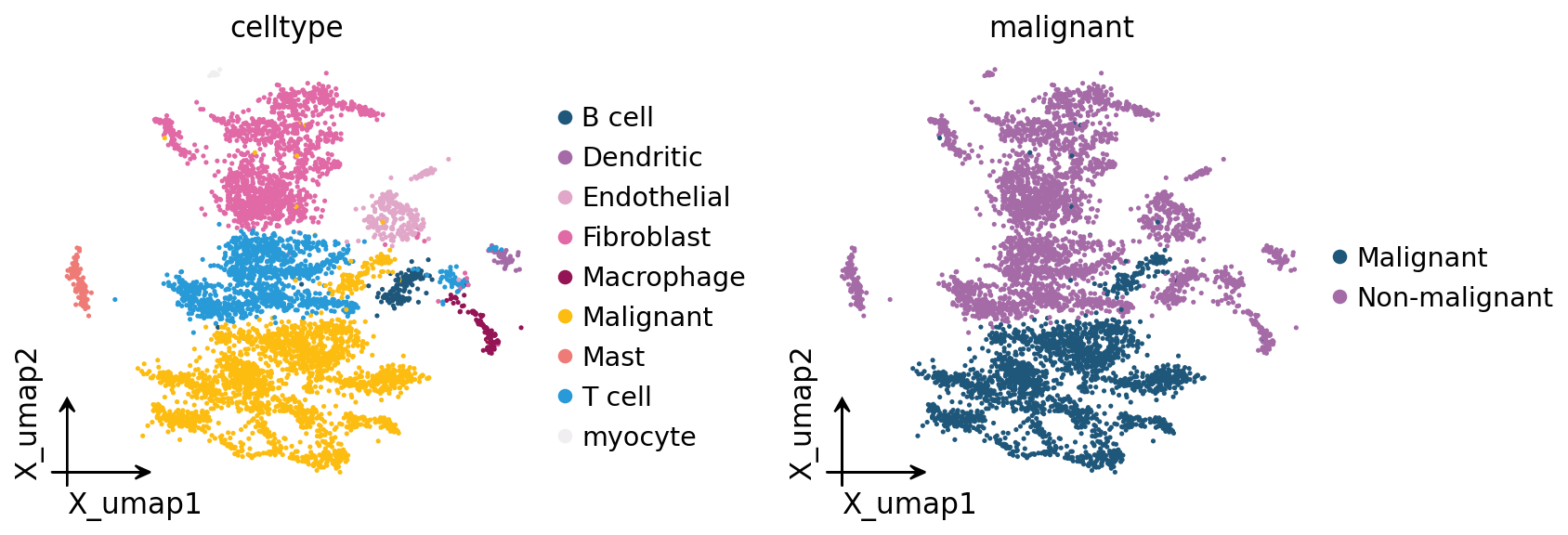
The Puram et al. 2017 head-and-neck squamous-cell-carcinoma atlas (GSE103322) — 5,578 single cells from 19 patients, the very dataset Xiao 2019 analysed. Expression is log2(TPM/10+1); each cell is annotated as malignant or as a stromal / immune cell type.
adata = ov.datasets.metabolism_hnsc()
adata
🔍 Downloading data to ./data/hnsc_puram2017_full.h5ad
⚠️ File ./data/hnsc_puram2017_full.h5ad already exists
AnnData object with n_obs × n_vars = 5578 × 23686
    obs: 'patient', 'malignant', 'celltype', 'lymph_node', 'maxima_enzyme'
    uns: 'dataset', 'expression_units'
adata.obs['celltype'].value_counts()
celltype
Malignant      2215
Fibroblast     1440
T cell         1237
Endothelial     260
B cell          138
Mast            120
Macrophage       98
Dendritic        51
myocyte          19
Name: count, dtype: int64
Part.3 Embedding#
A standard embedding for visualisation — the data is already
log-normalised, so we select highly variable genes, scale, and run
PCA / neighbours / UMAP with ov.pp.
ov.pp.highly_variable_genes(adata, n_top_genes=2000)
adata.raw = adata
hvg = adata[:, adata.var.highly_variable].copy()
ov.pp.scale(hvg)
ov.pp.pca(hvg, layer='scaled', n_pcs=30)
🔍 Highly Variable Genes Selection:
   Method: seurat
   Target genes: 2,000
📊 Top 2,000 genes correspond to normalized dispersion cutoff: 1.1786

✅ HVG Selection Completed Successfully!
   ✓ Selected: 2,000 highly variable genes out of 23,686 total (8.4%)
   ✓ Results added to AnnData object:
     • 'highly_variable': Boolean vector (adata.var)
     • 'means': Float vector (adata.var)
     • 'dispersions': Float vector (adata.var)
     • 'dispersions_norm': Float vector (adata.var)

╭─ SUMMARY: highly_variable_genes ───────────────────────────────────╮
│  Duration: 0.7612s                                                 │
│  Shape:    5,578 x 23,686 (Unchanged)                              │
│                                                                    │
│  CHANGES DETECTED                                                  │
│  ────────────────                                                  │
│  ● VAR    │ ✚ dispersions (float)                                  │
│           │ ✚ dispersions_norm (float)                             │
│           │ ✚ highly_variable (bool)                               │
│           │ ✚ means (float)                                        │
│                                                                    │
│  ● UNS    │ ✚ _ov_provenance                                       │
│           │ ✚ hvg                                                  │
│                                                                    │
╰────────────────────────────────────────────────────────────────────╯
╭─ SUMMARY: scale ───────────────────────────────────────────────────╮
│  Duration: 0.7233s                                                 │
│  Shape:    5,578 x 2,000 (Unchanged)                               │
│                                                                    │
│  CHANGES DETECTED                                                  │
│  ────────────────                                                  │
│  ● UNS    │ ✚ REFERENCE_MANU                                       │
│           │ ✚ status                                               │
│           │ ✚ status_args                                          │
│                                                                    │
│  ● LAYERS │ ✚ scaled (array, 5578x2000)                            │
│                                                                    │
╰────────────────────────────────────────────────────────────────────╯
computing PCA🔍
    with n_comps=30
   🖥️ Using sklearn PCA for CPU computation
   🖥️ sklearn PCA backend: CPU computation
   📊 PCA input data type: ArrayView, shape: (5578, 2000), dtype: float32
🔧 PCA solver used: covariance_eigh
    finished✅ (2.44s)

╭─ SUMMARY: pca ─────────────────────────────────────────────────────╮
│  Duration: 2.4514s                                                 │
│  Shape:    5,578 x 2,000 (Unchanged)                               │
│                                                                    │
│  CHANGES DETECTED                                                  │
│  ────────────────                                                  │
│  ● UNS    │ ✚ pca                                                  │
│           │ └─ params: {'zero_center': True, 'use_highly_variable': Tr...│
│           │ ✚ scaled|original|cum_sum_eigenvalues                  │
│           │ ✚ scaled|original|pca_var_ratios                       │
│                                                                    │
│  ● OBSM   │ ✚ X_pca (array, 5578x30)                               │
│           │ ✚ scaled|original|X_pca (array, 5578x30)               │
│                                                                    │
╰────────────────────────────────────────────────────────────────────╯
ov.pp.neighbors(hvg, n_neighbors=15, n_pcs=30,
                use_rep='scaled|original|X_pca')
ov.pp.umap(hvg)
adata.obsm['X_umap'] = hvg.obsm['X_umap']
🖥️ Using Scanpy CPU to calculate neighbors...

🔍 K-Nearest Neighbors Graph Construction:
   Mode: cpu
   Neighbors: 15
   Method: umap
   Metric: euclidean
   Representation: scaled|original|X_pca
   PCs used: 30
   🔍 Computing neighbor distances...
🔍 Computing connectivity matrix...
   💡 Using UMAP-style connectivity
✓ Graph is fully connected

✅ KNN Graph Construction Completed Successfully!
   ✓ Processed: 5,578 cells with 15 neighbors each
   ✓ Results added to AnnData object:
     • 'neighbors': Neighbors metadata (adata.uns)
     • 'distances': Distance matrix (adata.obsp)
     • 'connectivities': Connectivity matrix (adata.obsp)

╭─ SUMMARY: neighbors ───────────────────────────────────────────────╮
│  Duration: 13.2005s                                                │
│  Shape:    5,578 x 2,000 (Unchanged)                               │
│                                                                    │
│  CHANGES DETECTED                                                  │
│  ────────────────                                                  │
│  ● UNS    │ ✚ neighbors                                            │
│           │ └─ params: {'n_neighbors': 15, 'method': 'umap', 'random_s...│
│                                                                    │
│  ● OBSP   │ ✚ connectivities (sparse matrix, 5578x5578)            │
│           │ ✚ distances (sparse matrix, 5578x5578)                 │
│                                                                    │
╰────────────────────────────────────────────────────────────────────╯
🔍 [2026-05-22 06:44:23] Running UMAP in 'cpu' mode...
🖥️ Using Scanpy CPU UMAP...

🔍 UMAP Dimensionality Reduction:
   Mode: cpu
   Method: umap
   Components: 2
   Min distance: 0.5
{'n_neighbors': 15, 'method': 'umap', 'random_state': 0, 'metric': 'euclidean', 'use_rep': 'scaled|original|X_pca', 'n_pcs': 30}
   🔍 Computing UMAP parameters...
   🔍 Computing UMAP embedding (classic method)...
✅ UMAP Dimensionality Reduction Completed Successfully!
   ✓ Embedding shape: 5,578 cells × 2 dimensions
   ✓ Results added to AnnData object:
     • 'X_umap': UMAP coordinates (adata.obsm)
     • 'umap': UMAP parameters (adata.uns)
✅ UMAP completed successfully.

╭─ SUMMARY: umap ────────────────────────────────────────────────────╮
│  Duration: 1.3319s                                                 │
│  Shape:    5,578 x 2,000 (Unchanged)                               │
│                                                                    │
│  CHANGES DETECTED                                                  │
│  ────────────────                                                  │
│  ● UNS    │ ✚ umap                                                 │
│           │ └─ params: {'a': 0.5830300199950147, 'b': 1.334166993228519}│
│                                                                    │
│  ● OBSM   │ ✚ X_umap (array, 5578x2)                               │
│                                                                    │
╰────────────────────────────────────────────────────────────────────╯
ov.pl.embedding(adata, basis='X_umap', color=['celltype', 'malignant'],
                frameon='small', wspace=0.5)
Part.4 Score the metabolic landscape#
ov.single.Metabolism(method='scmetabolism') scores all 85 KEGG
metabolic pathways for every cell with the AUCell enrichment scorer.
The result lands in adata.obsm['X_metabolism'] — a 5,578 x 85
cell-by-pathway activity matrix.
met = ov.single.Metabolism(adata, method='scmetabolism')
met.run(score_method='AUCell', metabolism_type='KEGG')
<omicverse.single._metabolism.Metabolism at 0x7f46fa9584f0>
adata.obsm['X_metabolism'].shape # cells x KEGG metabolic pathways
(5578, 85)
Part.5 Malignant cells are the most metabolically active#
Xiao 2019’s headline result: against the bulk-tumour view, single
cells reveal that malignant cells up-regulate far more metabolic
pathways than any stromal or immune population. We test it with
ov.single.differential_metabolism — a Mann-Whitney test of every
pathway’s activity, malignant vs. non-malignant cells.
deg = ov.single.differential_metabolism(
    adata, groupby='malignant', group1='Malignant')
up = deg.query('padj < 0.05 and log2fc > 0')
print(f'{len(up)} of {len(deg)} KEGG pathways up-regulated in malignant cells')
53 of 85 KEGG pathways up-regulated in malignant cells
deg.head(8) # the most malignant-skewed metabolic pathways
| feature | mean1 | mean2 | log2fc | statistic | pval | padj | direction | |
|---|---|---|---|---|---|---|---|---|
| 0 | Glycolysis / Gluconeogenesis | 0.148391 | 0.089109 | 0.735763 | 6778325.0 | 0.0 | 0.0 | up |
| 1 | Pentose phosphate pathway | 0.106197 | 0.056830 | 0.902011 | 5944860.0 | 0.0 | 0.0 | up |
| 2 | Oxidative phosphorylation | 0.230178 | 0.122040 | 0.915394 | 6899061.5 | 0.0 | 0.0 | up |
| 3 | Folate biosynthesis | 0.070516 | 0.025385 | 1.473938 | 6044921.0 | 0.0 | 0.0 | up |
| 4 | Pyrimidine metabolism | 0.057207 | 0.036858 | 0.634212 | 6047366.5 | 0.0 | 0.0 | up |
| 5 | Cysteine and methionine metabolism | 0.093844 | 0.057375 | 0.709856 | 6207366.0 | 0.0 | 0.0 | up |
| 6 | Purine metabolism | 0.054976 | 0.038136 | 0.527640 | 6223389.5 | 0.0 | 0.0 | up |
| 7 | Phenylalanine metabolism | 0.099794 | 0.044781 | 1.156077 | 6432450.0 | 0.0 | 0.0 | up |
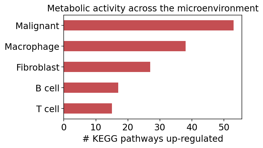
How does that compare across the microenvironment? We count the significantly up-regulated pathways for each cell type in turn. Xiao 2019 found malignant cells far ahead of every stromal and immune population — the metabolic activity of the tumour compartment that bulk RNA-seq averages away.
import pandas as pd

n_up = {ct: len(ov.single.differential_metabolism(
            adata, groupby='celltype', group1=ct)
        .query('padj < 0.05 and log2fc > 0'))
        for ct in ['Malignant', 'Fibroblast', 'Macrophage', 'B cell', 'T cell']}
pd.Series(n_up).sort_values(ascending=False)
Malignant     53
Macrophage    38
Fibroblast    27
B cell        17
T cell        15
dtype: int64
import matplotlib.pyplot as plt

ax = pd.Series(n_up).sort_values().plot.barh(color='#C44E52', figsize=(5, 3))
ax.set_xlabel('# KEGG pathways up-regulated')
ax.set_title('Metabolic activity across the microenvironment')
plt.show()
Part.6 Metabolic heterogeneity within the tumour#
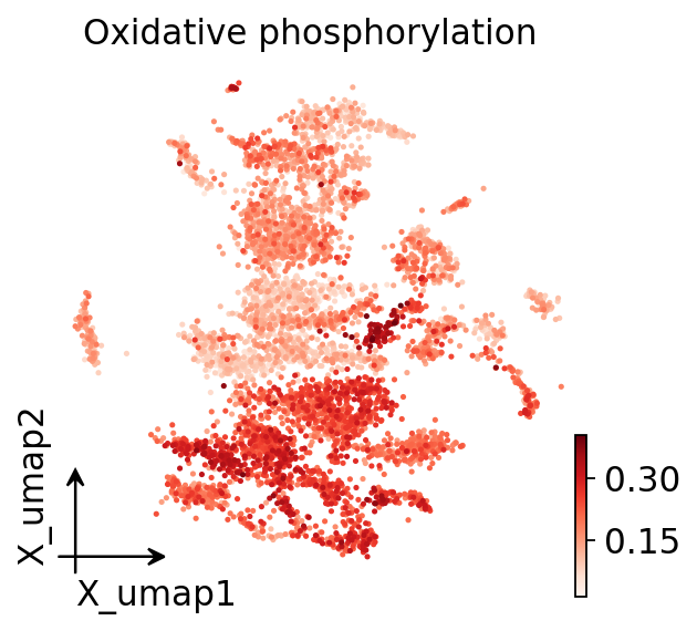
Xiao 2019 highlighted mitochondrial / oxidative-phosphorylation programs as a major source of intratumoural metabolic heterogeneity — even within one compartment, cells differ in energy metabolism. Projected onto the UMAP, OXPHOS activity is far from uniform across the tumour:
met.to_obs('Oxidative phosphorylation')
ov.pl.embedding(adata, basis='X_umap', color='Oxidative phosphorylation',
                cmap='Reds', frameon='small')
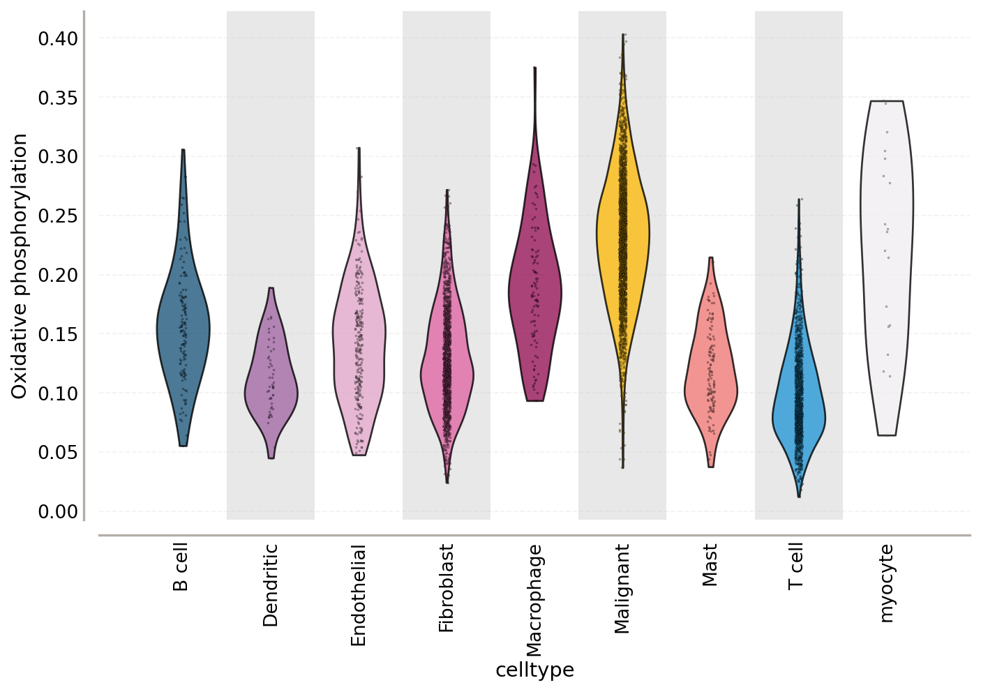
Resolved by cell type, OXPHOS varies both between cell types and within them — the spread inside the malignant violin is intratumoural metabolic heterogeneity:
ov.pl.violin(adata, keys='Oxidative phosphorylation',
             groupby='celltype', rotation=90)
<Axes: xlabel='celltype', ylabel='Oxidative phosphorylation'>
Part.7 Hypoxia, glycolysis and oxidative phosphorylation#
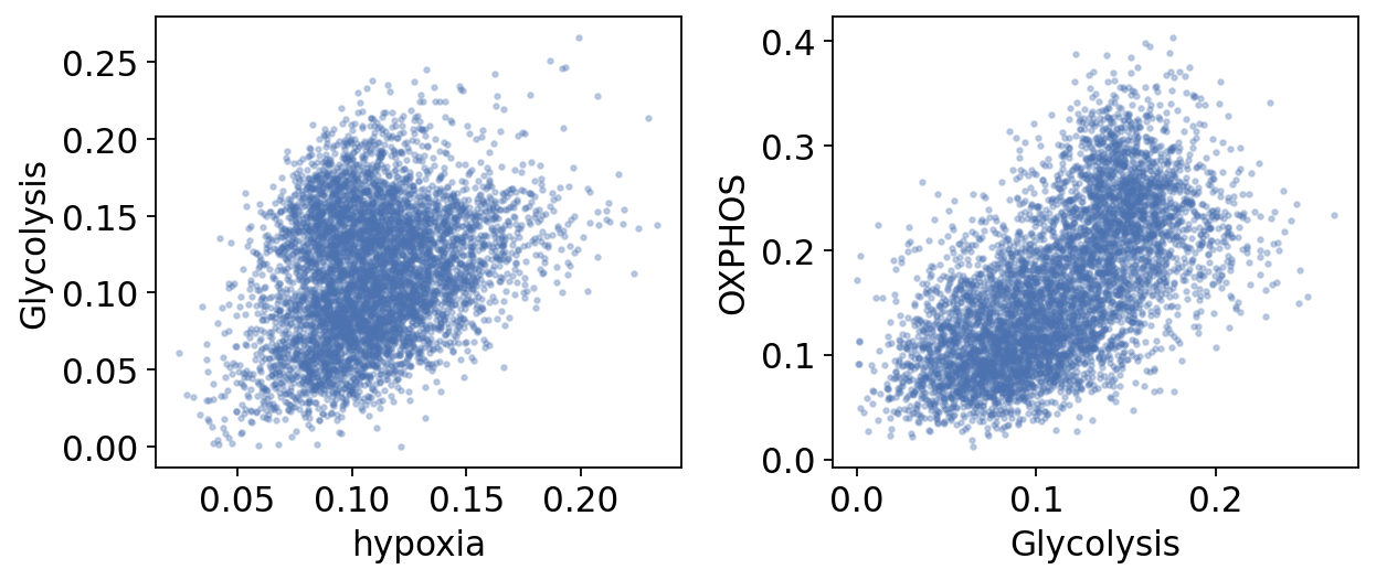
The classic Warburg picture casts the two energy programs as a trade-off — glycolysis on, OXPHOS off. Single-cell resolution tells a subtler story (Xiao 2019). We score each cell for the HALLMARK hypoxia signature and correlate it with both energy pathways.
sigs = ov.utils.geneset_prepare(
    ov.utils.predefined_signatures['hallmark'], organism='Human')
ov.es.aucell(adata, signatures={'hypoxia': sigs['HALLMARK_HYPOXIA']})
╭─ SUMMARY: aucell ──────────────────────────────────────────────────╮
│  Duration: 9.0969s                                                 │
│  Shape:    5,578 x 23,686 (Unchanged)                              │
│                                                                    │
│  CHANGES DETECTED                                                  │
│  ────────────────                                                  │
│  ● OBSM   │ ✚ score_aucell (dataframe, 5578x1)                     │
│                                                                    │
╰────────────────────────────────────────────────────────────────────╯
scores = met.get()
energy = pd.DataFrame({
    'hypoxia': adata.obsm['score_aucell']['hypoxia'].to_numpy(),
    'Glycolysis': scores['Glycolysis / Gluconeogenesis'].to_numpy(),
    'OXPHOS': scores['Oxidative phosphorylation'].to_numpy()})
energy.corr().round(2)
| hypoxia | Glycolysis | OXPHOS | |
|---|---|---|---|
| hypoxia | 1.00 | 0.29 | -0.02 |
| Glycolysis | 0.29 | 1.00 | 0.62 |
| OXPHOS | -0.02 | 0.62 | 1.00 |
Two real signals emerge: glycolysis rises modestly with the hypoxia score — the canonical HIF axis — and glycolysis and OXPHOS are positively correlated, co-elevated rather than traded off, exactly the Xiao 2019 point. OXPHOS on its own does not track hypoxia in this cohort.
fig, axes = plt.subplots(1, 2, figsize=(8, 3.5))
for ax, (x, y) in zip(axes, [('hypoxia', 'Glycolysis'),
                              ('Glycolysis', 'OXPHOS')]):
    ax.scatter(energy[x], energy[y], s=4, alpha=0.3, color='#4C72B0')
    ax.set(xlabel=x, ylabel=y)
plt.tight_layout(); plt.show()
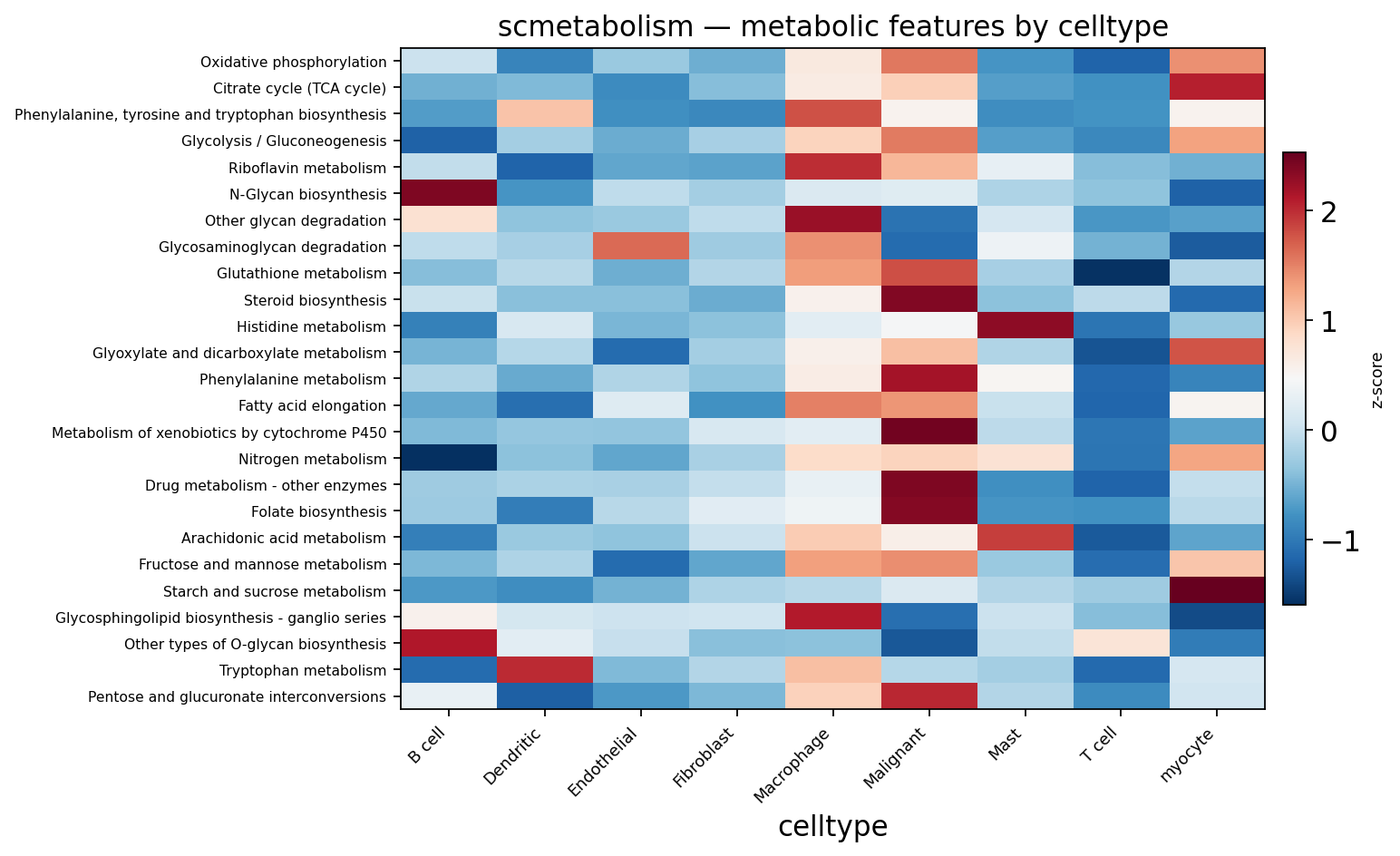
Part.8 Cell-type-specific metabolic programs#
Beyond the malignant compartment, each microenvironment cell type
runs its own metabolic program — ov.pl.metabolism_heatmap averages
pathway activity within each cell type and keeps the most
discriminating, non-redundant pathways.
ov.pl.metabolism_heatmap(adata, groupby='celltype', n_features=25)
<Axes: title={'center': 'scmetabolism — metabolic features by celltype'}, xlabel='celltype'>
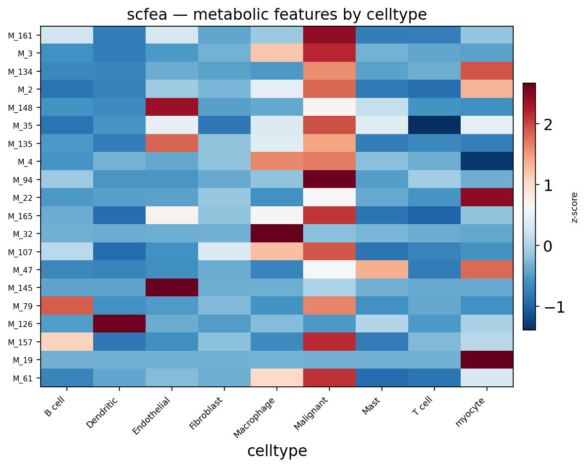
Part.9 Metabolic flux with scFEA#
Pathway activity reads gene expression; metabolic flux asks how fast each reaction actually runs. scFEA estimates flux through ~168 metabolic modules with a graph neural network constrained by metabolite mass-balance. Flux estimation is heavier than scoring, so we run it on a 400-cell subsample as a complementary view.
import numpy as np
idx = np.random.default_rng(0).choice(adata.n_obs, 400, replace=False)
sub = adata[idx].copy()
flux = ov.single.Metabolism(sub, method='scfea')
flux.run(n_epoch=25, verbose=False)
<omicverse.single._metabolism.Metabolism at 0x7f465c11b130>
ov.pl.metabolism_heatmap(sub, groupby='celltype', n_features=20)
<Axes: title={'center': 'scfea — metabolic features by celltype'}, xlabel='celltype'>
Recap — a metabolic landscape, reproduced#
Running ov.single.Metabolism on the Puram 2017 HNSC atlas recovers
the core conclusions of Xiao et al. 2019:
finding |
this analysis |
|---|---|
malignant cells up-regulate the most metabolic pathways |
counted with |
OXPHOS heterogeneity within the tumour |
the OXPHOS UMAP + per-cell-type violin |
glycolysis tracks hypoxia; glycolysis & OXPHOS co-elevated |
the hypoxia / glycolysis / OXPHOS correlation table |
cell types run distinct programs |
the cell-type x pathway heatmap |
The third paradigm, Compass constraint-based reaction flux, is
available as ov.single.Metabolism(method='compass') — it needs a
commercial LP solver and is run offline. For metabolite-mediated
cell-cell communication in this same tumour, see the companion
tutorial Metabolite cell-cell communication with MEBOCOST.