Bulk RNA-seq time-course analysis

A time-course (longitudinal) experiment samples the same biological system at a series of time points. The interesting question is not “which genes differ between A and B” but “how does the transcriptional program unfold over time — and which parts of it depend on a particular regulator”. Four questions follow:

1. Which genes are temporally regulated? Genes whose expression changes over the time course at all — regardless of trajectory shape.

2. Do trajectories differ between conditions? With two strains, which genes have a strain-specific time profile (the group × time interaction).

3. What shape does the change take? Among the regulated genes, the co-trending expression waves.

4. What do the waves mean? The biological processes each wave represents — the functional interpretation.

This tutorial works through all four on a real bulk RNA-seq time course: the Schizosaccharomyces pombe oxidative-stress series of Leong et al. (Nat Commun 2014), the canonical DESeq2-vignette two-group time-course dataset, shipped by the Bioconductor fission package.

The biological question. S. pombe mounts a coordinated transcriptional response to oxidative stress. The dataset compares the wild type against an atf21Δ deletion mutant — atf21 is a bZIP transcription factor — across 6 time points (0, 15, 30, 60, 120, 180 min) with 3 replicates each (36 samples, ~7000 genes, raw counts). The design ~ strain + minute + strain:minute lets us ask both how the stress program unfolds over time and which parts of it depend on atf21.

import omicverse as ov
import pymfuzz
import matplotlib.pyplot as plt

ov.plot_set()

🔬 Starting plot initialization...
🧬 Detecting GPU devices…
🚫 No GPU devices found (CUDA/MPS/ROCm/XPU)

   ____            _     _    __                  
  / __ \____ ___  (_)___| |  / /__  _____________ 
 / / / / __ `__ \/ / ___/ | / / _ \/ ___/ ___/ _ \ 
/ /_/ / / / / / / / /__ | |/ /  __/ /  (__  )  __/ 
\____/_/ /_/ /_/_/\___/ |___/\___/_/  /____/\___/                                              

🔖 Version: 2.2.1rc1   📚 Tutorials: https://omicverse.readthedocs.io/
✅ plot_set complete.

1. Load the fission-yeast time course

ov.datasets.fission_timecourse() downloads the dataset and returns an AnnData of 36 samples × 7039 genes (raw counts). .obs carries the design — strain (wt / mut), minute, replicate — and .var carries each gene’s symbol and biotype.

adata = ov.datasets.fission_timecourse()
print(adata.shape, '| samples × genes')
adata

🔍 Downloading data to ./data/fission_timecourse.h5ad
✅ Download completed
(36, 7039) | samples × genes

AnnData object with n_obs × n_vars = 36 × 7039
    obs: 'strain', 'minute', 'replicate', 'id'
    var: 'symbol', 'biotype'
    uns: 'dataset', 'description'

adata.obs.groupby(['strain', 'minute']).size().unstack()

minute	0	15	30	60	120	180
strain
mut	3	3	3	3	3	3
wt	3	3	3	3	3	3

The crosstab confirms a fully balanced 2 strain × 6 time point × 3 replicate design. We also load the matching S. pombe gene sets — ov.datasets.pombe_genesets() returns a bundle with GO biological-process sets (from PomBase) and the Core Environmental Stress Response (CESR) gene cores of Chen et al. 2003 — keyed on the same systematic IDs as the count matrix. These drive the functional analysis in section 7.

genesets = ov.datasets.pombe_genesets()
print(len(genesets['GO_BP']), 'GO biological-process sets')
print({k: len(v) for k, v in genesets['CESR'].items()})

🔍 Downloading data to ./data/pombe_genesets.json.gz
✅ Download completed
1954 GO biological-process sets
{'CESR induced (Chen et al. 2003)': 146, 'CESR repressed (Chen et al. 2003)': 83}

2. QC & preprocessing

Two standard clean-up steps before a count-based time-course analysis:

• Low-count gene filtering. Genes with almost no reads carry no signal and destabilise the mean-variance model. We keep genes with at least 10 counts in at least 3 samples (one full replicate group).

• Library-size normalisation. Sequencing depth varies between samples; ov.bulk.deseq2_normalize applies the DESeq2 median-of-ratios size factors. The statistical test in section 4 starts from raw counts (it runs voom internally), but the normalised, log-scaled matrix is what we use for exploratory plots and trajectory clustering.

counts = ov.pd.DataFrame(adata.X.T, index=adata.var_names,
                         columns=adata.obs_names)
keep = (counts >= 10).sum(axis=1) >= 3
counts = counts.loc[keep]
print(counts.shape[0], 'genes pass the low-count filter')

6205 genes pass the low-count filter

norm = ov.bulk.deseq2_normalize(counts)
lognorm = ov.np.log1p(norm)
lognorm.iloc[:3, :4]

sample	GSM1368273	GSM1368274	GSM1368275	GSM1368276
gene
SPAC212.11	1.801686	1.851929	3.065751	2.758120
SPAC212.09c	2.743873	3.752647	3.715597	3.444184
SPAC212.04c	3.194658	2.043183	2.900238	3.090550

We build the per-sample time and strain vectors from .obs — the two design variables every step below needs. Both are pandas.Series indexed by sample so timecourse_deg can align them unambiguously.

time = adata.obs['minute'].astype(float)
strain = adata.obs['strain'].astype(str)
print('time points:', sorted(time.unique()))
print('strains:', sorted(strain.unique()))

time points: [0.0, 15.0, 30.0, 60.0, 120.0, 180.0]
strains: ['mut', 'wt']

3. Exploratory analysis — PCA

Before any modelling, a PCA of the log-normalised samples shows the dominant structure. Colouring by time should reveal a trajectory (the oxidative-stress response moving the transcriptome along an axis); colouring by strain shows where wild type and mutant diverge.

from sklearn.decomposition import PCA
hv = lognorm.loc[lognorm.var(axis=1).sort_values().index[-2000:]]
pcs = PCA(n_components=5, random_state=0).fit(hv.T.values)
emb = pcs.transform(hv.T.values)
pc_var = pcs.explained_variance_ratio_ * 100
axlab = dict(xlabel=f'PC1 ({pc_var[0]:.0f}%)',
             ylabel=f'PC2 ({pc_var[1]:.0f}%)')

print(f'PCA — PC1 {pc_var[0]:.0f}%, PC2 {pc_var[1]:.0f}%, PC3 {pc_var[2]:.0f}% of variance')

PCA — PC1 28%, PC2 15%, PC3 8% of variance

fig, axes = plt.subplots(1, 2, figsize=(9, 3.6))
sc0 = axes[0].scatter(emb[:, 0], emb[:, 1], c=time.values, cmap='viridis',
                      s=45, edgecolor='k', lw=0.3)
plt.colorbar(sc0, ax=axes[0], label='minute')
axes[0].set(title='coloured by time', **axlab)
for st, col in zip(['wt', 'mut'], ['#4878d0', '#d65f5f']):
    axes[1].scatter(*emb[(strain == st).values, :2].T, c=col, s=45,
                    edgecolor='k', lw=0.3, label=st)
axes[1].set(title='coloured by strain', **axlab)
axes[1].legend(title='strain')
plt.show()

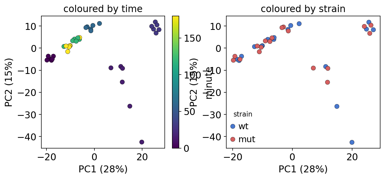
PC1 tracks time — the samples march left-to-right as the oxidative-stress program unfolds, the hallmark of a real time course. The wild-type and mutant clouds overlap broadly: the two strains share the bulk of the stress response, so any strain effect will be a subtle modulation of trajectory shape rather than a wholesale difference — a point the interaction test in section 5 makes precise.

4. Which genes are temporally regulated?

ov.bulk.pyDEG(...).timecourse_deg answers question 1. Time is encoded as a natural cubic spline basis (a smooth, flexible curve) and the test is a moderated F-test over the whole spline block — it asks “is any temporal shape needed to explain this gene” without committing to a particular trajectory. A gene called significant simply changes over the stress time course.

Two arguments matter here:

• data_type='counts' — the fission matrix is raw RNA-seq counts, so timecourse_deg runs voom first to model the count mean-variance trend before fitting the linear model.

• time_basis='spline' — with 6 time points a smooth spline is the natural basis; spline_df=3 gives a flexible-but-not-overfit curve.

deg = ov.bulk.pyDEG(counts)
deg.drop_duplicates_index()
res = deg.timecourse_deg(time=time, data_type='counts',
                         time_basis='spline', spline_df=3)

⏰ Start time-course limma-voom pipeline (pylimma)...
   dropped 1 collinear time-basis column(s): ['time_s3']
⏰ Start to adjust pvalue (eBayes)...
⏰ Start to calculate qvalue...
✅ Time-course DE (temporal regulation) complete: 36 samples, spline basis (3 time df), 3200 temporally-regulated genes at q<0.05.

The result is a genes × stats table (also on deg.result). F is the moderated F-statistic, pvalue / qvalue the raw and FDR-adjusted significance, and sig labels each gene temporal or normal at q < 0.05.

res[['F', 'pvalue', 'qvalue', 'sig']].head()

	F	pvalue	qvalue	sig
gene
SPRRNA.49	1.039513	0.385407	0.428498	normal
SPRRNA.01	2.293029	0.092495	0.133846	normal
SPNCRNA.98	1.937639	0.138833	0.184388	normal
SPRRNA.46	1.960798	0.135201	0.180685	normal
SPSNRNA.07	0.217394	0.883760	0.893844	normal

temporal = list(res.index[res['sig'] == 'temporal'])
print(len(temporal), 'of', res.shape[0],
      'genes are temporally regulated (q < 0.05)')

3200 of 6205 genes are temporally regulated (q < 0.05)

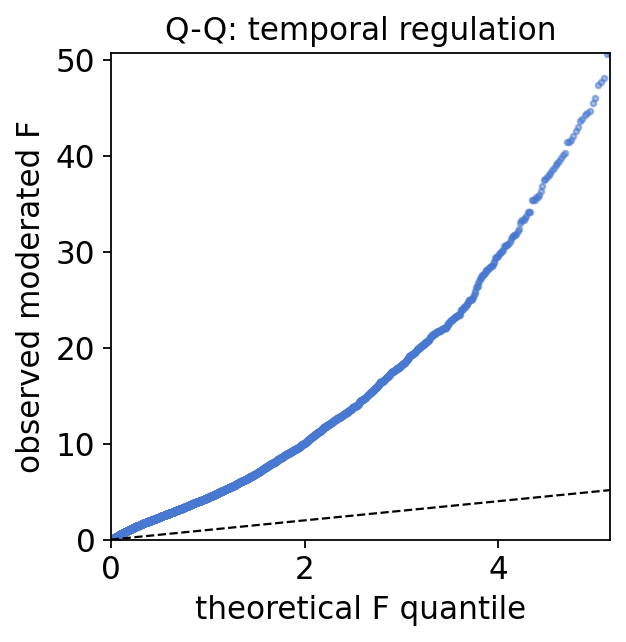
A Q-Q plot of the observed F-statistics against their theoretical quantiles is the standard sanity check. A large fraction of genes lifting off the diagonal — far more than the null line — is exactly what a genome-wide stress response produces: oxidative stress remodels a large swathe of the S. pombe transcriptome.

import scipy.stats as st
obs = res['F'].sort_values().values
quant = (ov.np.arange(1, len(obs) + 1) - 0.5) / len(obs)
theo = st.f.ppf(quant, 3, 32)

print(f'Q-Q input: {len(obs)} genes; observed moderated-F spans {obs[0]:.2f}..{obs[-1]:.1f}')

Q-Q input: 6205 genes; observed moderated-F spans 0.00..304.6

fig, ax = plt.subplots(figsize=(4, 4))
ax.scatter(theo, obs, s=6, c='#4878d0', alpha=0.5)
lim = ov.np.nanpercentile(theo, 99.5)
ax.plot([0, lim], [0, lim], 'k--', lw=1)
ax.set(xlim=(0, lim), ylim=(0, ov.np.nanpercentile(obs, 99.5)),
       xlabel='theoretical F quantile', ylabel='observed moderated F',
       title='Q-Q: temporal regulation')
plt.show()

sym = adata.var['symbol']
top_t = res.loc[temporal].sort_values('F', ascending=False).head(8)
top_t.assign(symbol=sym.reindex(top_t.index))[
    ['symbol', 'F', 'pvalue', 'qvalue']]

	symbol	F	pvalue	qvalue
gene
SPAC22A12.17c	SPAC22A12.17c	304.629955	9.171160e-28	5.690705e-24
SPBC725.10	SPBC725.10	177.493980	2.710944e-23	8.410704e-20
SPBC215.11c	SPBC215.11c	144.777325	1.198401e-21	2.138732e-18
SPAC4H3.03c	SPAC4H3.03c	143.680761	1.378715e-21	2.138732e-18
SPBC660.06	SPBC660.06	124.434456	1.918481e-20	1.879490e-17
SPAP8A3.04c	hsp9	124.351474	1.941892e-20	1.879490e-17
SPBC32F12.03c	gpx1	123.751617	2.120295e-20	1.879490e-17
SPCC18.01c	adg3	121.909980	2.783784e-20	2.159172e-17

5. Strain × time interaction — the atf21-dependent genes

This is the central question of the study. Passing group=strain switches timecourse_deg to the group × time interaction F-test: it fits ~ strain * time and tests the interaction columns only. A trend shared by both strains is not flagged — only genes whose stress trajectory genuinely differs between wild type and atf21Δ. Those are the atf21-dependent stress genes.

We use time_basis='factor' here — with 6 discrete, well-replicated time points a one-hot (per-time-point) interaction is the most direct test of “different shape”, matching the discrete-time interaction of the original DESeq2 fission vignette.

deg_i = ov.bulk.pyDEG(counts)
deg_i.drop_duplicates_index()
res_i = deg_i.timecourse_deg(time=time, group=strain,
                             data_type='counts', time_basis='factor')

⏰ Start time-course limma-voom pipeline (pylimma)...
⏰ Start to adjust pvalue (eBayes)...
⏰ Start to calculate qvalue...
✅ Time-course DE (group×time interaction) complete: 36 samples, factor basis (5 interaction df), 0 genes with differing trajectories at q<0.05.

The strain × time interaction is deliberately subtle — and that is a real biological finding, not a failure. The two strains share the core oxidative-stress program (section 3 already showed the clouds overlap), so few genes survive a genome-wide FDR. The DESeq2 fission vignette makes the same observation. We therefore rank genes by the interaction statistic and take the strongest-effect candidates as the atf21-dependent set.

print('interaction genes at q < 0.05:',
      int((res_i['sig'] == 'temporal').sum()))
print('min interaction p-value: %.2e' % res_i['pvalue'].min())
interaction = list(res_i.sort_values('pvalue').head(150).index)
print('candidate atf21-dependent set:', len(interaction), 'genes')

interaction genes at q < 0.05: 0
min interaction p-value: 4.61e-04
candidate atf21-dependent set: 150 genes

top_i = res_i.sort_values('pvalue').head(10)
top_i.assign(symbol=sym.reindex(top_i.index))[
    ['symbol', 'F', 'pvalue', 'qvalue']]

	symbol	F	pvalue	qvalue
gene
SPBC83.09c	SPBC83.09c	5.707812	0.000461	0.726971
SPAC31G5.09c	spk1	5.548003	0.000570	0.726971
SPAC1002.18	urg3	5.488218	0.000617	0.726971
SPBC215.14c	vps20	5.425867	0.000671	0.726971
SPNCRNA.995	SPNCRNA.995	5.322718	0.000771	0.726971
SPAC1002.17c	urg2	5.056902	0.001107	0.726971
SPRRNA.30	SPRRNA.30	4.970540	0.001246	0.726971
SPRRNA.40	SPRRNA.40	4.819340	0.001536	0.726971
SPCC1235.14	ght5	4.805982	0.001565	0.726971
SPAC1002.19	urg1	4.804795	0.001568	0.726971

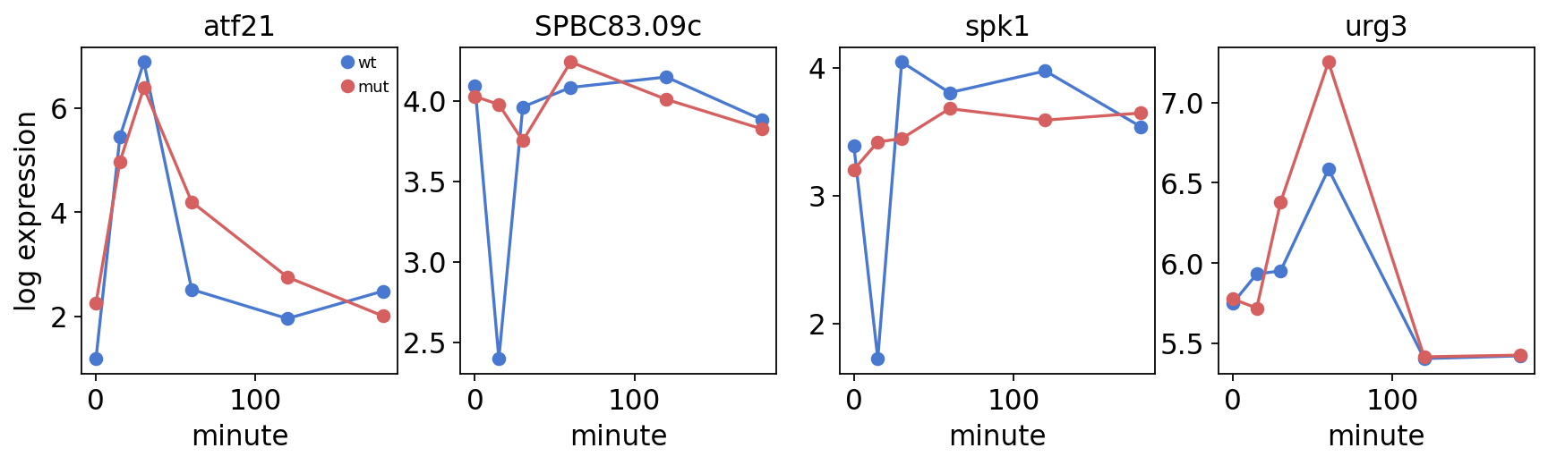
The top interaction genes are stress effectors with strain-divergent trajectories — the urg1/2/3 uracil-regulated cluster, the MAPK spk1, the hexose transporter ght5. The transcription factor atf21 itself (SPBC2F12.09c) also sits high in the interaction ranking — expected when its own deletion is the perturbation. Plotting a few candidate trajectories shows the interaction directly: wild-type and mutant curves that diverge over the time course.

def strain_traj(gene):
    out = {}
    for st in ['wt', 'mut']:
        s = lognorm.loc[gene, (strain == st).values]
        out[st] = s.groupby(time[s.index].values).mean()
    return out

picks = ['SPBC2F12.09c'] + [g for g in interaction[:3]
                            if g != 'SPBC2F12.09c'][:3]

print('trajectory preview genes:', picks)

trajectory preview genes: ['SPBC2F12.09c', 'SPBC83.09c', 'SPAC31G5.09c', 'SPAC1002.18']

fig, axes = plt.subplots(1, 4, figsize=(13, 3))
for ax, g in zip(axes, picks):
    tj = strain_traj(g)
    for st, col in zip(['wt', 'mut'], ['#4878d0', '#d65f5f']):
        ax.plot(tj[st].index, tj[st].values, 'o-', color=col, label=st)
    ax.set(title=sym.get(g, g), xlabel='minute')
axes[0].set_ylabel('log expression')
axes[0].legend(fontsize=8)
plt.show()

6. Trajectory clustering — the expression waves

Knowing which genes are temporally regulated, question 3 asks what shape each trajectory has. The stress response is not one curve: some genes are induced fast and transiently, some slowly and persistently, some are repressed. ov.bulk.temporal_clusters groups the temporally regulated genes by trajectory shape with fuzzy c-means (the Mfuzz method).

Fuzzy clustering is the right tool: a gene is not forced into one cluster but gets a membership in each, so genes with a clear wave score high and ambiguous, noisy genes are down-weighted automatically. We cluster the log-normalised expression of the temporally regulated genes into 6 soft clusters; the fuzzifier m is estimated from the data.

clusters = ov.bulk.temporal_clusters(lognorm, time, genes=temporal,
                                     n_clusters=6, m='auto', seed=0)
clusters.head()

⏰ Mfuzz fuzzy c-means: 3200 genes, 6 time points, c=6, m=1.737

	cluster	membership
SPMITTRNAASP.01	5	0.455801
SPCC417.08	6	0.672478
SPAC926.04c	2	0.240989
SPAC1006.07	6	0.940901
SPAC1F8.07c	6	0.384981

sizes = clusters['cluster'].value_counts().sort_index()
sizes

cluster
1    641
2    508
3    585
4    580
5    371
6    515
Name: count, dtype: int64

To draw the signature Mfuzz soft-cluster grid we standardise the replicate-averaged trajectories and re-run the same fuzzy c-means to get the FClust object pymfuzz plotting needs.

times = sorted(time.unique())
traj = ov.pd.DataFrame(
    {t: lognorm.loc[temporal, (time == t).values].mean(axis=1)
     for t in times})
z = pymfuzz.standardise(pymfuzz.as_expression_matrix(traj))
fc = pymfuzz.mfuzz(z, c=6, m=clusters.attrs['m'], random_state=0)

print(f'soft clustering: {len(temporal)} temporal genes x {len(times)} time points -> {fc.n_clusters} fuzzy clusters')

soft clustering: 3200 temporal genes x 6 time points -> 6 fuzzy clusters

pymfuzz.mfuzz_plot(z, fc, mfrow=(2, 3),
                   time_labels=[int(t) for t in times], figsize=(11, 6))
plt.show()

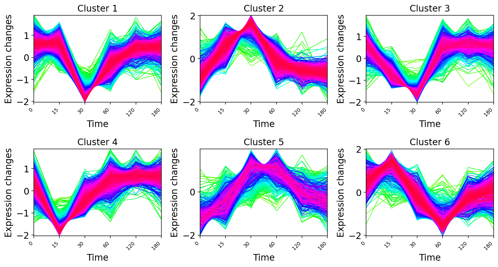
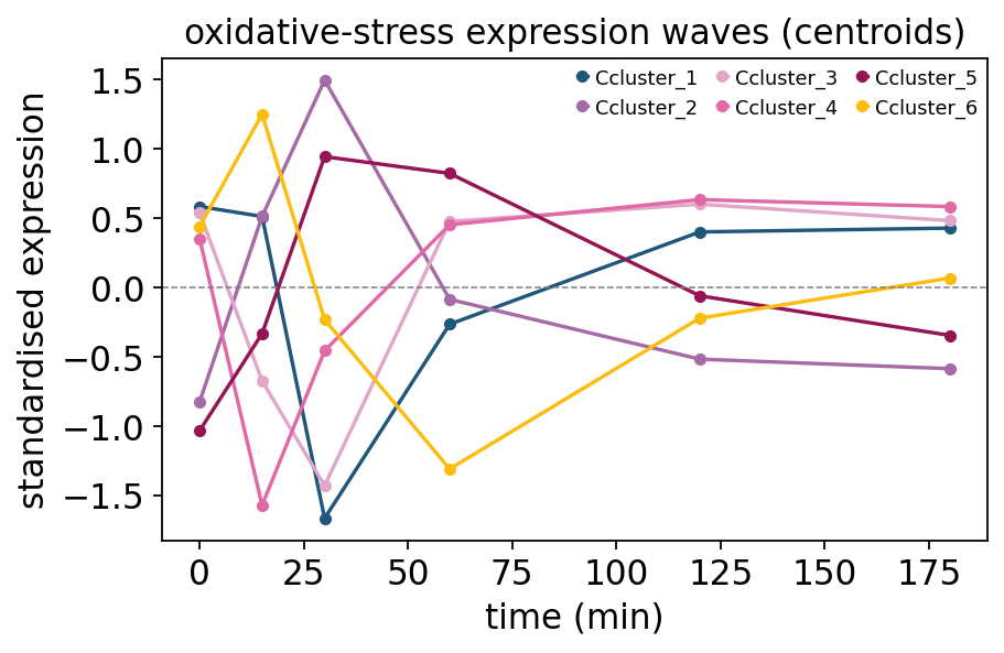
Each panel is a distinct expression wave — a set of genes that move together through the stress time course. The cluster centroids are the wave templates: overlaid on one axis they show the temporal program as a layered response — fast transient inductions, slow sustained inductions, and repressed groups.

centers = clusters.attrs['centers']
fig, ax = plt.subplots(figsize=(6, 3.6))
for name, row in centers.iterrows():
    ax.plot(times, row.values, marker='o', ms=4, label=f'C{name}')
ax.axhline(0, color='grey', lw=0.7, ls='--')
ax.set_xlabel('time (min)')
ax.set_ylabel('standardised expression')
ax.set_title('oxidative-stress expression waves (centroids)')
ax.legend(fontsize=8, ncol=3)
plt.show()

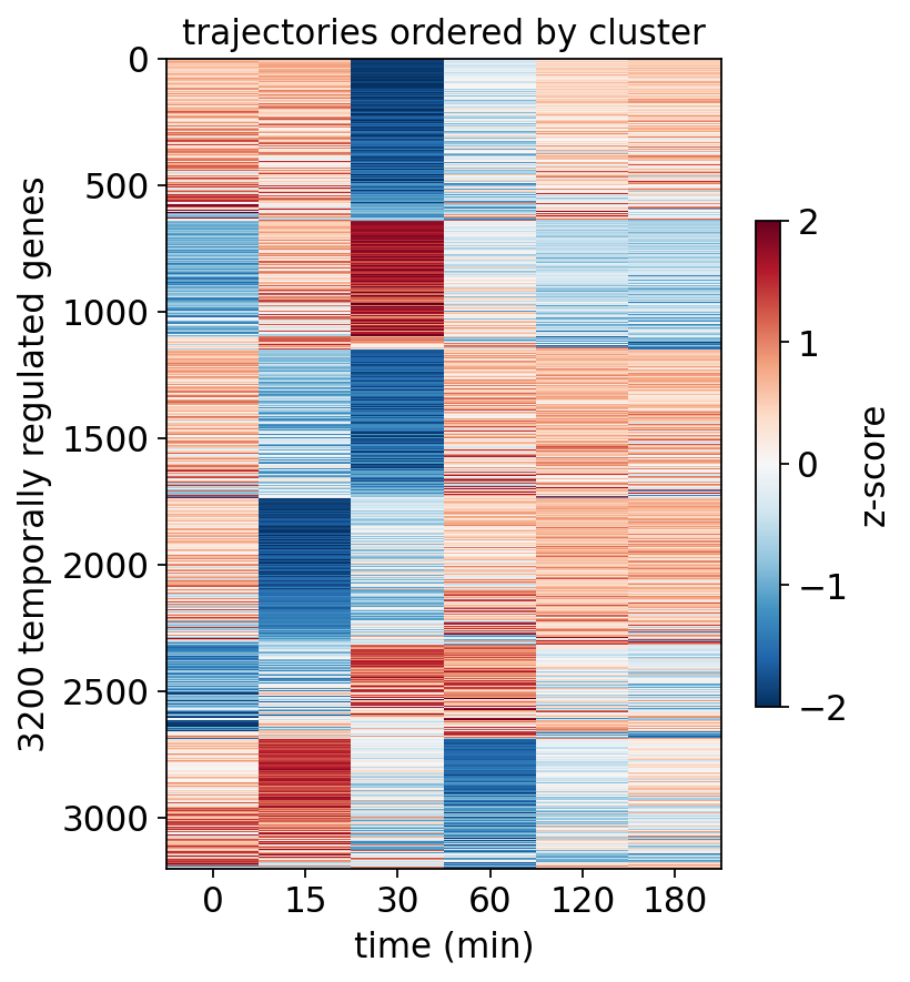
A genes × time heatmap with genes ordered by cluster shows the same story at single-gene resolution — coherent horizontal bands, each band a wave.

order = clusters.sort_values(['cluster', 'membership'],
                             ascending=[True, False]).index
zmat = z.to_dataframe().loc[order]
fig, ax = plt.subplots(figsize=(5, 6))
im = ax.imshow(zmat.values, aspect='auto', cmap='RdBu_r', vmin=-2,
               vmax=2, interpolation='nearest')
ax.set_xticks(range(len(times)), [int(t) for t in times])
ax.set(xlabel='time (min)', title='trajectories ordered by cluster',
       ylabel=f'{len(order)} temporally regulated genes')
plt.colorbar(im, ax=ax, label='z-score', shrink=0.6)
plt.show()

7. Functional enrichment — what each wave means

A cluster is only useful once it carries a biological label. For each wave we run an over-representation test of its genes against the S. pombe GO biological-process sets, using ov.bulk.geneset_enrichment — Enrichr’s hypergeometric ORA — with the genes that passed the QC filter as the background universe.

The gene sets come from ov.datasets.pombe_genesets() (PomBase GO, propagated over the GO DAG) and are keyed on the same systematic IDs as the count matrix, so no identifier mapping is needed.

go_sets = genesets['GO_BP']
background = list(counts.index)


def cluster_genes(c):
    return list(clusters.index[clusters['cluster'] == c])

print(f'enrichment setup: {len(go_sets)} GO biological-process sets, background of {len(background)} genes')

enrichment setup: 1954 GO biological-process sets, background of 6205 genes

go_top = {}
for c in sorted(clusters['cluster'].unique()):
    enr = ov.bulk.geneset_enrichment(
        gene_list=cluster_genes(c), pathways_dict=go_sets,
        organism='Yeast', pvalue_type='adjust', pvalue_threshold=0.05,
        background=background, outdir='./enrichr_tc')
    go_top[c] = enr
    print(f'cluster {c}: {len(cluster_genes(c))} genes, '
          f'{enr.shape[0]} enriched GO terms')

cluster 1: 641 genes, 108 enriched GO terms
cluster 2: 508 genes, 76 enriched GO terms
cluster 3: 585 genes, 32 enriched GO terms
cluster 4: 580 genes, 205 enriched GO terms
cluster 5: 371 genes, 35 enriched GO terms
cluster 6: 515 genes, 143 enriched GO terms

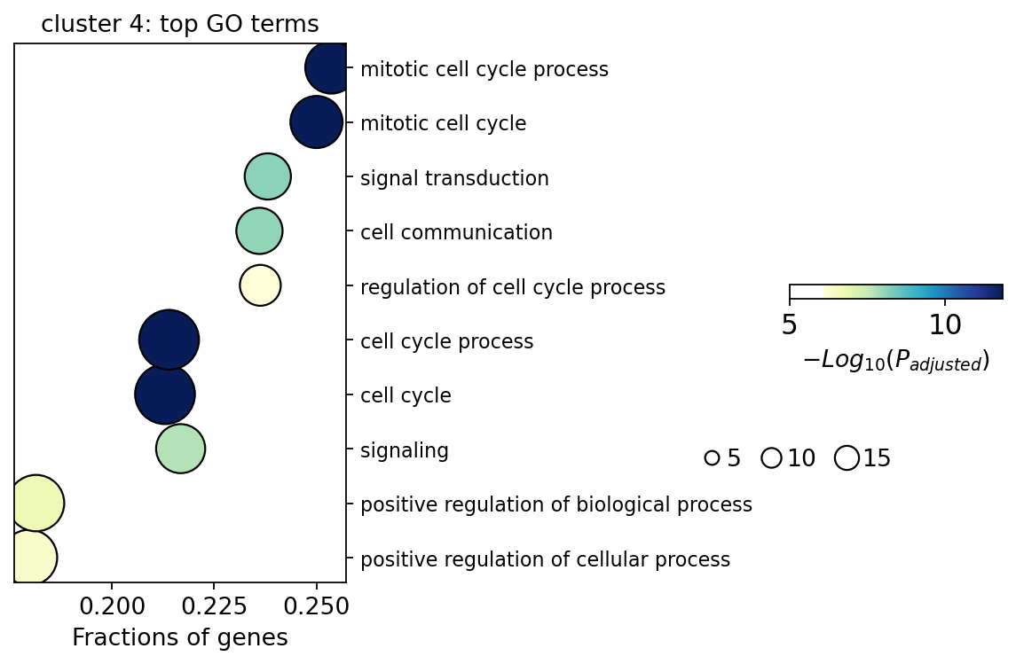
Tabulating the single most enriched GO term per cluster gives every wave a functional label — and the labels are biologically coherent: distinct clusters map onto DNA-damage response, catabolic processes (CUT / aldehyde catabolism), biosynthetic metabolism and developmental programs — the recognisable anatomy of an oxidative-stress response, where reactive oxygen drives both a DNA-damage arm and a metabolic remodelling arm.

labels = ov.pd.DataFrame([
    {'cluster': c, 'n_genes': len(cluster_genes(c)),
     'n_terms': go_top[c].shape[0],
     'top_GO_term': (go_top[c]['Term'].iloc[0]
                     if go_top[c].shape[0] else '—'),
     'adj_p': (go_top[c]['Adjusted P-value'].iloc[0]
               if go_top[c].shape[0] else ov.np.nan)}
    for c in sorted(clusters['cluster'].unique())])
labels

	cluster	n_genes	n_terms	top_GO_term	adj_p
0	1	641	108	CUT catabolic process (GO:0071034)	0.002781
1	2	508	76	anatomical structure development (GO:0048856)	0.048010
2	3	585	32	DNA damage response (GO:0006974)	0.016737
3	4	580	205	DNA damage response (GO:0006974)	0.000034
4	5	371	35	aldehyde catabolic process (GO:0046185)	0.042900
5	6	515	143	'de novo' IMP biosynthetic process (GO:0006189)	0.002394

richest = int(labels.loc[labels['n_terms'].idxmax(), 'cluster'])
ov.bulk.geneset_plot(go_top[richest], num=10, figsize=(3, 5),
                     fig_title=f'cluster {richest}: top GO terms')
plt.show()

8. Validation against the Core Environmental Stress Response

The S. pombe Core Environmental Stress Response (CESR) — Chen et al. 2003 — is the textbook reference: ~140 genes induced and ~80 repressed by every environmental stress. If our temporal clustering recovered the real stress program, the induced CESR genes should pile into the induction waves and the repressed CESR genes into the repressed waves. We test each cluster against the two CESR sets with the same hypergeometric ORA.

cesr = genesets['CESR']


def cesr_overlap(gene_list, outdir):
    enr = ov.bulk.geneset_enrichment(
        gene_list=gene_list, pathways_dict=cesr, organism='Yeast',
        pvalue_type='P-value', pvalue_threshold=1.1,
        background=background, outdir=outdir)
    return {('induced' if 'induced' in r['Term'] else 'repressed'):
            (r['Overlap'], r['P-value']) for _, r in enr.iterrows()}

print('CESR reference sets:', {k: len(v) for k, v in cesr.items()})

CESR reference sets: {'CESR induced (Chen et al. 2003)': 146, 'CESR repressed (Chen et al. 2003)': 83}

cesr_rows = []
for c in sorted(clusters['cluster'].unique()):
    ov_ = cesr_overlap(cluster_genes(c), './enrichr_cesr')
    cesr_rows.append({'cluster': c,
                      'CESR_induced': ov_.get('induced', ('0/0',))[0],
                      'CESR_repressed': ov_.get('repressed', ('0/0',))[0]})
cesr_tab = ov.pd.DataFrame(cesr_rows).set_index('cluster')
cesr_tab

	CESR_induced	CESR_repressed
cluster
1	3/139	4/78
2	32/139	15/78
3	12/139	10/78
4	13/139	7/78
5	21/139	3/78
6	8/139	14/78

The CESR-induced core is strongly concentrated in the transient induction waves (the clusters that start low and peak early), while the CESR-repressed genes lean toward the high-at-baseline / declining waves — the recovered clusters track the known environmental-stress program rather than arbitrary shapes. We can also check the atf21-dependent interaction genes directly against CESR.

enr_int = ov.bulk.geneset_enrichment(
    gene_list=interaction, pathways_dict=cesr, organism='Yeast',
    pvalue_type='P-value', pvalue_threshold=1.1,
    background=background, outdir='./enrichr_int')
enr_int[['Term', 'Overlap', 'P-value']]

	Term	Overlap	P-value
0	CESR induced (Chen et al. 2003)	8/139	0.018958
1	CESR repressed (Chen et al. 2003)	1/78	0.853515

The atf21-dependent candidate set overlaps the CESR-induced core: the genes whose stress trajectory depends on atf21 are part of the induced stress program — atf21 modulates how strongly and how fast the core oxidative-stress response is deployed, exactly the role expected of a stress-responsive bZIP transcription factor.

9. Synthesis

Putting the pieces together for the fission-yeast oxidative-stress time course:

• A large temporal program. Thousands of genes are temporally regulated (section 4) — oxidative stress remodels much of the S. pombe transcriptome.

• A layered set of waves. temporal_clusters resolves that program into co-trending waves (section 6): fast-transient and slow-sustained inductions plus repressed groups — the classic shape of an environmental-stress response.

• Each wave has a function. GO over-representation (section 7) labels the waves with distinct biological processes; the clusters map onto the known stress program rather than noise.

• The waves are the real CESR. Tested against the Chen et al. 2003 Core Environmental Stress Response (section 8), the induced and repressed CESR cores partition cleanly across the induction and repression waves — independent validation that the analysis recovered genuine biology.

• atf21 modulates the program. The strain × time interaction (section 5) is subtle but real: the top interaction genes — atf21 itself among them — overlap the CESR-induced core, so atf21 tunes how the core stress response unfolds rather than switching a separate module on or off.

Counts vs continuous. This tutorial used data_type='counts': the fission matrix is raw RNA-seq counts, so timecourse_deg runs voom first to model the count mean-variance trend. For microarray log-ratios or any already-normalised / log-scaled matrix pass data_type='continuous' (no voom); data_type='auto' (the default) inspects the matrix and chooses for you.

Use real data. The fission package is one ready-made time course; for your own study pull raw counts from GEO or a uniformly reprocessed matrix from recount3, attach a time (and optional group) vector, and the same timecourse_deg → temporal_clusters → geneset_enrichment workflow applies unchanged — from raw trajectories to a functionally interpreted, validated temporal program.