HEST-FM — pathology foundation model + ridge head

The HEST benchmark (Jaume et al., NeurIPS 2024 Spotlight) showed that the strongest recipe for predicting spatial expression from H&E is also the simplest: take a pretrained pathology foundation model (UNI / CONCH / Virchow2 / GigaPath / CTransPath / …), extract per-tile features, fit one ridge regression per gene on a paired Visium slide, and predict on new tiles. With ≥1 paired reference slide this beats most end-to-end deep architectures while training in seconds.

ov.space.histo.predict_expression(method='hest_fm') implements this recipe end-to-end on top of LazySlide / WSIData.

Why “with paired reference”? A single Visium slide gives you 3–5 k (tile, expression) training pairs, more than enough to fit a stable linear head per gene. This is in contrast to STPath / STFlow which are pretrained cross-cohort and can run zero-shot on a brand-new H&E.

This notebook uses the all-public CTransPath backbone so it runs without any HuggingFace gating. For higher accuracy swap in fm_backbone='uni2', 'conch_v1.5', 'virchow2', or 'gigapath' once you have access.

Environment

import warnings
warnings.filterwarnings('ignore')

import omicverse as ov
import lazyslide as zs

ov.utils.ov_plot_set()
print('omicverse', ov.__version__, '| lazyslide', zs.__version__)

🔬 Starting plot initialization...
🧬 Detecting GPU devices…
✅ NVIDIA CUDA GPUs detected: 1
    • [CUDA 0] NVIDIA H100 80GB HBM3
      Memory: 79.1 GB | Compute: 9.0

   ____            _     _    __                  
  / __ \____ ___  (_)___| |  / /__  _____________ 
 / / / / __ `__ \/ / ___/ | / / _ \/ ___/ ___/ _ \ 
/ /_/ / / / / / / / /__ | |/ /  __/ /  (__  )  __/ 
\____/_/ /_/ /_/_/\___/ |___/\___/_/  /____/\___/                                              

🔖 Version: 2.2.1rc1   📚 Tutorials: https://omicverse.readthedocs.io/
✅ plot_set complete.

omicverse 2.2.1rc1 | lazyslide 0.9.2

How the WSI flows through LazySlide

ov.space.histo does not re-implement WSI handling — it wraps LazySlide (the scverse-aligned WSI toolkit) and lifts its WSIData container into the omicverse namespace. Concretely:

omicverse call	LazySlide / wsidata under the hood
ov.space.histo.open_wsi(path)	wsidata.open_wsi(path) — returns a WSIData (a SpatialData subclass) wrapping the slide reader (openslide / tiffslide / bioformats) and a thumbnail
ov.space.histo.tile(wsi, …)	zs.pp.find_tissues + zs.pp.tile_tissues — writes tissue contours to wsi.shapes['tissues'] and a tile grid to wsi.shapes['tiles']
ov.space.histo.embed(wsi, model=…)	zs.tl.feature_extraction — runs the chosen pathology FM on every tile and stores features as wsi.tables['{model}_tiles'] (an AnnData with one row per tile)
ov.space.histo.predict_expression(wsi, method=…)	omicverse-specific: writes another AnnData table wsi.tables['{method}_tiles'] with predicted gene expression

The WSIData API surface stays available — drop down to zs.pp.* / zs.tl.* / zs.pl.* whenever you need finer control than the convenience wrappers expose.

Inputs HEST-FM expects

Two objects, both in the same pixel coordinate frame:

• reference — paired Visium AnnData

  • reference.X (n_spots × n_genes) — raw spot counts

  • reference.obsm['spatial'] (n_spots × 2) — spot pixel centroids in the H&E frame

  • reference.uns['spatial'][lib]['scalefactors']['spot_diameter_fullres'] — the spot diameter in full-resolution pixels; HEST-FM uses it as the side length of the reference patches it cuts out under each spot

• wsi — wsidata.WSIData wrapping the H&E used in the reference, plus optionally any query H&E you want to predict on. In this tutorial both reference and query are the same slide, but you can also tile and embed a different slide as the query as long as its tile features come from the same fm_backbone.

Both objects are returned together by load_breast(); the next markdown cell shows how to assemble them for your own data.

Model weights & cache layout

HEST-FM uses one pretrained foundation-model checkpoint (the patch encoder) and trains a tiny ridge head per gene on the user’s reference. Everything is auto-downloaded on first use; nothing needs manual setup beyond the install.

What	From	To	Size	Gated?
ctranspath patch encoder (default)	LazySlide model registry → HF RendeiroLab/LazySlide-models-gpl	$HF_HOME/hub/ (default ~/.cache/huggingface/hub)	~100 MB	no
reference spot-patch features (per slide / backbone)	computed once	$OV_HISTO_CACHE/ref_features/{backbone}_{slide_stem}_n{n_spots}.h5ad	~10–50 MB	—
query tile features (per slide / tile-grid / backbone)	computed once	$OV_HISTO_CACHE/tile_features/{backbone}_{slide_stem}_{tile_key}_n{n_tiles}.h5ad	~10–50 MB	—
per-gene Ridge head	trained at predict time	in-memory, not persisted	—	—

$OV_HISTO_CACHE defaults to ~/.cache/omicverse/histo. Override the location with OV_HISTO_CACHE=/some/path (recommended on HPC: point it at a scratch filesystem). Override the HuggingFace location with HF_HOME=/some/path (default ~/.cache/huggingface).

Swapping to a more accurate gated backbone — set fm_backbone='uni2' (or 'conch_v1.5', 'virchow2', 'gigapath', 'h-optimus-1') once you have HuggingFace access. Request access on the model card, then huggingface-cli login once on this machine. LazySlide handles the gated download for you.

Load the demo dataset

ov.space.histo.load_breast() downloads and caches the 10x Visium Breast Cancer Block A Section 1 sample under $OV_HISTO_CACHE/he_zoo/visium_breast (~1.7 GB on disk; one-time).

adata, wsi = ov.space.histo.load_breast()
adata

AnnData object with n_obs × n_vars = 3798 × 36601
    obs: 'in_tissue', 'array_row', 'array_col'
    var: 'gene_ids', 'feature_types', 'genome'
    uns: 'spatial', 'histo'
    obsm: 'spatial'

wsi

WSI: /scratch/users/steorra/cache/omicverse_histo/he_zoo/visium_breast/V1_Breast_Cancer_Block_A_Section_1_image.tif
Reader: tiffslide
Dimensions: 24240×24240 (h×w), 1 Pyramid
Pixel physical size: 0.31 MPP

SpatialData object
└── Images
      └── 'wsi_thumbnail': DataArray[cyx] (3, 2000, 2000)
with coordinate systems:
    ▸ 'global', with elements:
        wsi_thumbnail (Images)

Loading your own data

For a real Space Ranger output:

adata, wsi = ov.space.histo.read_visium_with_image(
    visium_path='/path/to/spaceranger/outs',
    image_path='/path/to/full_resolution_HE.tif',
    count_file='filtered_feature_bc_matrix.h5',
)

The helper delegates to scverse-stack readers and wsidata.open_wsi for you and derives wsi.properties.mpp from spot_diameter_fullres so the downstream backends know the physical scale. Predicting on a different slide than the reference works the same way — just pass that slide’s wsi (after tile() + embed()) as the first argument while keeping reference= pointed at the Visium AnnData you already have.

Tile and embed the WSI

• tile(wsi, tile_px=224, mpp=0.5) runs LazySlide’s find_tissues + tile_tissues. tile_px=224 matches every pathology FM’s input size, and mpp=0.5 (µm / pixel) is the standard “pathology zoom” level — each 224-pixel patch covers ~112 µm of tissue, roughly twice a Visium spot’s footprint.

• embed(wsi, model='ctranspath', batch_size=16, num_workers=0) extracts per-tile features and writes them as wsi.tables['ctranspath_tiles'] (an AnnData with one row per tile and 768 feature columns). The on-disk cache key includes slide id, tile key, tile count, and backbone, so re-running this cell on the same WSI returns instantly.

ov.space.histo.tile(wsi, tile_px=224, mpp=0.5)
ov.space.histo.embed(wsi, model='ctranspath',
                     batch_size=16, num_workers=0)
print('tiles:', len(wsi.shapes['tiles']),
      '| feature table:', list(wsi.tables))

tiles: 1426 | feature table: ['ctranspath_tiles']

Fit a Ridge head on the reference and predict on the query

predict_expression(method='hest_fm', …) does the following under the hood:

1. cut out a 1-tile-per-spot grid on the reference WSI at tile_px = spot_diameter_fullres,

2. embed those reference patches with fm_backbone (cached to $OV_HISTO_CACHE/ref_features/),

3. PCA-project both reference and query embeddings to n_components dimensions,

4. fit one sklearn.linear_model.Ridge per requested gene on the reference, predict on the query tile features,

5. wrap predictions in an AnnData and store it as wsi.tables['hest_fm_tiles'].

Key parameters

• reference — paired Visium AnnData (required for hest_fm).

• genes=['EPCAM', …] — gene panel to predict. Pass None to predict all of reference.var_names.

• fm_backbone='ctranspath' — which pathology FM to extract features with. List all options with ov.space.histo.available_backbones().

• n_components=128 — PCA dimensionality. Smaller = faster + more regularised; larger = retain more FM signal at the cost of overfitting risk on small references.

• alpha=1.0 — Ridge regularisation strength. Increase if the head overfits (Pearson on held-out spots drops).

• head='ridge' — set to 'mlp' for a 2-layer GELU MLP fitted with AdamW; usually a small gain on dense panels, not worth the extra compute on a 5-gene panel.

Pre-staging the patch-encoder weights

HEST-FM downloads the chosen FM from the LazySlide registry on first use. To run air-gapped (or to use a checkpoint you’ve validated elsewhere) pass an explicit path:

pred = ov.space.histo.predict_expression(
    wsi, method='hest_fm', reference=adata,
    fm_backbone='ctranspath',
    fm_weight_path='/path/to/ctranspath.pth',  # skips HF download
    hf_token=None,                              # not needed when path is given
    cache_dir='/path/to/scratch/omicverse_histo',
)

genes = ['EPCAM', 'ERBB2', 'CD68', 'ACTA2', 'VIM']
pred = ov.space.histo.predict_expression(
    wsi,
    method='hest_fm',
    reference=adata,
    genes=genes,
    fm_backbone='ctranspath',
    n_components=128,
    alpha=1.0,
)
pred

AnnData object with n_obs × n_vars = 1426 × 5
    obs: 'tile_id', 'library_id'
    var: 'gene_ids', 'feature_types', 'genome'
    uns: 'histo'
    obsm: 'spatial'

Reading the output

pred is an AnnData whose rows are query tiles (NOT Visium spots) and whose columns are the requested genes:

• pred.X (n_tiles × n_genes) — log1p predicted expression, float32

• pred.var_names — the requested gene symbols

• pred.obsm['spatial'] (n_tiles × 2) — tile pixel centroids, ready for any spatial plotter

• pred.uns['histo'] — run metadata (method, fm_backbone, n_components, alpha, head)

print('shape       :', pred.shape)
print('var_names   :', list(pred.var_names))
print('coords range:', pred.obsm['spatial'].min(0), '→',
                       pred.obsm['spatial'].max(0))
print('metadata    :', pred.uns['histo'])

shape       : (1426, 5)
var_names   : ['EPCAM', 'ERBB2', 'CD68', 'ACTA2', 'VIM']
coords range: [4468.5 4355.5] → [22223.5 23521.5]
metadata    : {'method': 'hest_fm', 'fm_backbone': 'ctranspath', 'n_components': 128, 'alpha': 1.0, 'head': 'ridge'}

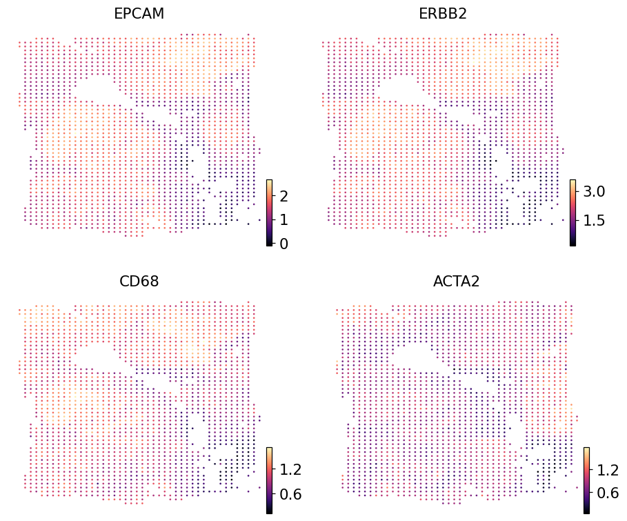
Visualise predictions on the tissue

Tile-pixel centroids are in obsm['spatial'], so any spatial plotter (ov.pl.embedding / ov.pl.spatial, zs.pl.tiles) works directly. For high tile counts (3k+) ov.pl.embedding is the fastest path; zs.pl.tiles(style='heatmap') is useful for publication-quality renders that paint the WSI under the patches.

ov.pl.embedding(pred, basis='spatial',
                color=['EPCAM', 'ERBB2', 'CD68', 'ACTA2'],
                cmap='magma', s=12, ncols=2, frameon=False)

Real Visium counts for the same genes

Render the same four genes from the paired Visium reference so they can be eyeballed against the predictions above. The reference is log1p-normalised (ov.pp.normalize_total + ov.pp.log1p) so the colour scale matches the predictor’s output.

ref = adata.copy()
ov.pp.normalize_total(ref, target_sum=1e4)
ov.pp.log1p(ref)
ov.pl.embedding(ref, basis='spatial',
                color=['EPCAM', 'ERBB2', 'CD68', 'ACTA2'],
                cmap='magma', s=24, ncols=2, frameon=False)

🔍 Count Normalization:
   Target sum: 10000.0
   Exclude highly expressed: False

✅ Count Normalization Completed Successfully!
   ✓ Processed: 3,798 cells × 36,601 genes
   ✓ Runtime: 0.06s

Per-gene scatter on Section 1 (training fit quality)

The ridge head was trained on Section 1’s spots, so this scatter shows the best-case fit — how well the model can reproduce its own training data. Tile and spot grids don’t coincide, so each Visium spot is matched to its nearest predicted tile before plotting. Pearson r is shown in the title; the dashed line is predicted = true.

import numpy as np, matplotlib.pyplot as plt
from scipy.spatial import cKDTree
from scipy.stats import pearsonr

spot_xy = adata.obsm['spatial']
tile_xy = pred.obsm['spatial']
nn = cKDTree(tile_xy).query(spot_xy, k=1)[1]

ref_X = adata[:, pred.var_names].X
ref_X = np.log1p(ref_X.toarray() if hasattr(ref_X, 'toarray') else ref_X)
pred_X = pred.X[nn]

fig, axes = plt.subplots(1, len(pred.var_names),
                         figsize=(3 * len(pred.var_names), 3))
for ax, g, i in zip(axes, pred.var_names, range(len(pred.var_names))):
    ax.scatter(ref_X[:, i], pred_X[:, i], s=4, alpha=0.4)
    r, _ = pearsonr(ref_X[:, i], pred_X[:, i])
    lo = float(min(ref_X[:, i].min(), pred_X[:, i].min()))
    hi = float(max(ref_X[:, i].max(), pred_X[:, i].max()))
    ax.plot([lo, hi], [lo, hi], 'k--', lw=0.8, alpha=0.5)
    ax.set_title(f'{g}: r={r:.2f}')
    ax.set_xlabel('Section 1 real log1p')
    ax.set_ylabel('HEST-FM prediction')
plt.tight_layout()

Held-out evaluation on a fresh slide (Section 2)

The Pearson table above mixes “training data” (the H&E patches the ridge head saw) with the comparison spots, so it overestimates real-world quality. To get an honest number, predict on Section 2 — the adjacent physical section of the same patient block, available from 10x as a second Visium dataset. Same anatomy, same staining batch, but every H&E pixel is genuinely new to the model.

load_breast(section=2) downloads it (~1.7 GB on first use, then cached) and returns the same (adata, wsi) shape as Section 1.

adata_s2, wsi_s2 = ov.space.histo.load_breast(section=2)
ov.space.histo.tile(wsi_s2, tile_px=224, mpp=0.5)
ov.space.histo.embed(wsi_s2, model='ctranspath',
                     batch_size=16, num_workers=0)
adata_s2, wsi_s2

(AnnData object with n_obs × n_vars = 3987 × 36601
    obs: 'in_tissue', 'array_row', 'array_col'
    var: 'gene_ids', 'feature_types', 'genome'
    uns: 'spatial', 'histo'
    obsm: 'spatial', WSI: /scratch/users/steorra/cache/omicverse_histo/he_zoo/visium_breast_s2/V1_Breast_Cancer_Block_A_Section_2_image.tif
Reader: tiffslide
Dimensions: 24240×24240 (h×w), 1 Pyramid
Pixel physical size: 0.3099797227629586 MPP
SpatialData object
├── Images
│     └── 'wsi_thumbnail': DataArray[cyx] (3, 2000, 2000)
├── Shapes
│     ├── 'tiles': GeoDataFrame shape: (1857, 3) (2D shapes)
│     └── 'tissues': GeoDataFrame shape: (1, 2) (2D shapes)
└── Tables
      └── 'ctranspath_tiles': AnnData (1857, 768)
with coordinate systems:
    ▸ 'global', with elements:
        wsi_thumbnail (Images), tiles (Shapes), tissues (Shapes))

Predict on Section 2’s tiles using the same call shape — only wsi= and the reference change.

pred_s2 = ov.space.histo.predict_expression(
    wsi_s2,                       # query: Section 2 H&E tiles
    method='hest_fm',
    reference=adata,              # train: Section 1 Visium spots
    genes=genes,                  # same 5-gene panel
    fm_backbone='ctranspath',
    n_components=128, alpha=1.0,
)
pred_s2

AnnData object with n_obs × n_vars = 1857 × 5
    obs: 'tile_id', 'library_id'
    var: 'gene_ids', 'feature_types', 'genome'
    uns: 'histo'
    obsm: 'spatial'

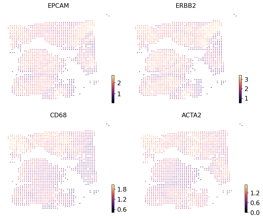
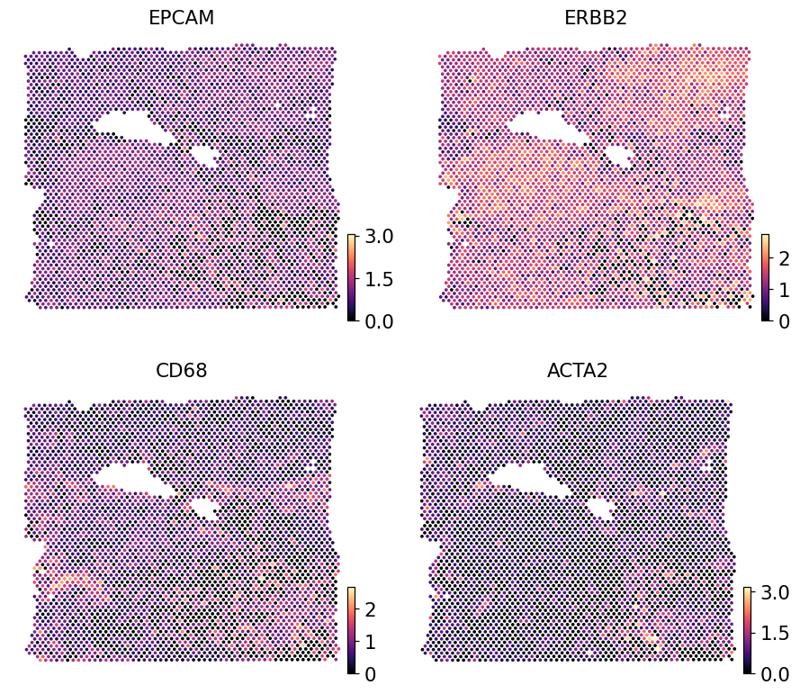
Spatial visualisation on Section 2 — prediction

Same ov.pl.embedding call as Section 1, just pointed at the held-out slide’s predicted AnnData.

ov.pl.embedding(pred_s2, basis='spatial',
                color=['EPCAM', 'ERBB2', 'CD68', 'ACTA2'],
                cmap='magma', s=12, ncols=2, frameon=False)

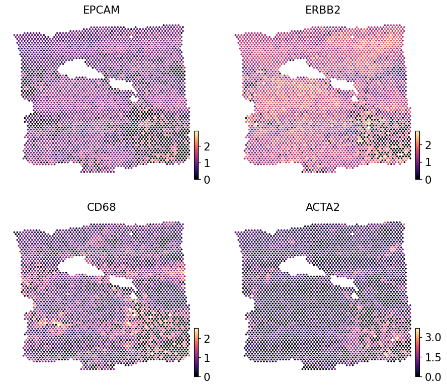
Spatial visualisation on Section 2 — real Visium counts

Section 2’s real Visium expression for the same panel; compare visually with the predicted maps above. Log1p-normalised so the colour scale matches the predictor’s output.

ref_s2 = adata_s2.copy()
ov.pp.normalize_total(ref_s2, target_sum=1e4)
ov.pp.log1p(ref_s2)
ov.pl.embedding(ref_s2, basis='spatial',
                color=['EPCAM', 'ERBB2', 'CD68', 'ACTA2'],
                cmap='magma', s=24, ncols=2, frameon=False)

🔍 Count Normalization:
   Target sum: 10000.0
   Exclude highly expressed: False

✅ Count Normalization Completed Successfully!
   ✓ Processed: 3,987 cells × 36,601 genes
   ✓ Runtime: 0.06s

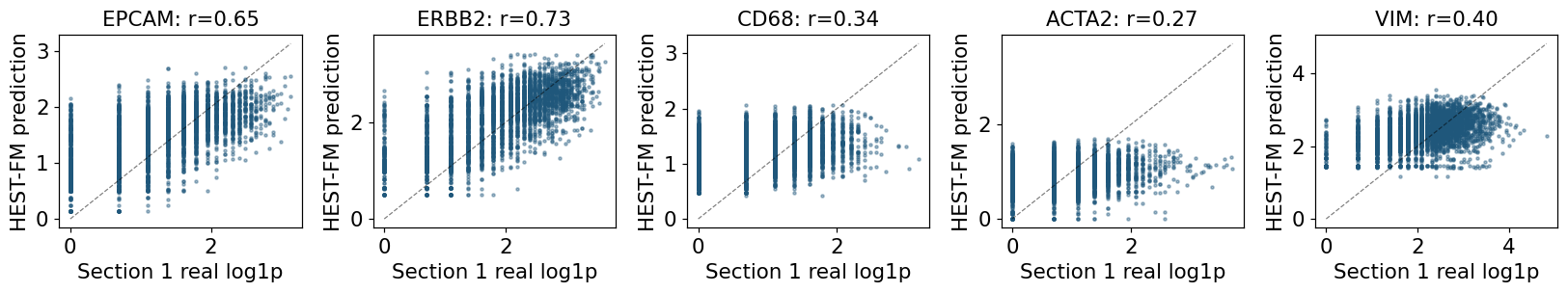
Per-gene scatter on Section 2 (truly held-out)

Match each Section 2 Visium spot to its nearest Section 2 predicted tile, scatter the real log1p expression against the prediction. Pearson r in the title.

import numpy as np, matplotlib.pyplot as plt
from scipy.spatial import cKDTree
from scipy.stats import pearsonr

spot_xy = adata_s2.obsm['spatial']
tile_xy = pred_s2.obsm['spatial']
nn = cKDTree(tile_xy).query(spot_xy, k=1)[1]

ref_X = adata_s2[:, pred_s2.var_names].X
ref_X = np.log1p(ref_X.toarray() if hasattr(ref_X, 'toarray') else ref_X)
pred_X = pred_s2.X[nn]

fig, axes = plt.subplots(1, len(pred_s2.var_names),
                         figsize=(3 * len(pred_s2.var_names), 3))
for ax, g, i in zip(axes, pred_s2.var_names, range(len(pred_s2.var_names))):
    ax.scatter(ref_X[:, i], pred_X[:, i], s=4, alpha=0.4)
    r, _ = pearsonr(ref_X[:, i], pred_X[:, i])
    lo = float(min(ref_X[:, i].min(), pred_X[:, i].min()))
    hi = float(max(ref_X[:, i].max(), pred_X[:, i].max()))
    ax.plot([lo, hi], [lo, hi], 'k--', lw=0.8, alpha=0.5)
    ax.set_title(f'{g}: r={r:.2f}')
    ax.set_xlabel('Section 2 real log1p')
    ax.set_ylabel('HEST-FM prediction')
plt.tight_layout()

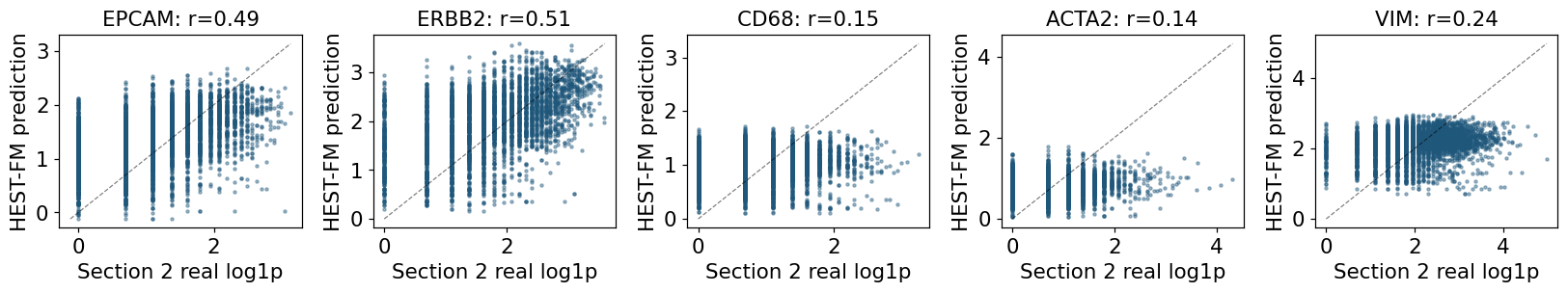
Reading the numbers — per-gene Pearson r ≈ 0.3–0.7 is typical for the all-public CTransPath backbone on a 5-gene panel. Two things noticeably move it up:

• swap fm_backbone='uni2' / 'virchow2' / 'gigapath' (gated, see model card) — typically +5-15% mean r;

• bump the panel size (HEST-Bench fits 50 HVG ridges per slide, which stabilises the alpha pick).

The dashed diagonal is predicted = true; the more the cloud hugs it, the better.

Where to go next

The predicted AnnData is interchangeable with a real Visium table, so downstream ov.space analyses just work:

ov.space.pySTAGATE(pred, n_domains=8, radius=20)   # spatial domains
pred = ov.space.svg(pred, mode='prost', n_svgs=200)  # spatially-variable genes
ov.pl.spatial(pred, color='STAGATE_domain')

Compare with the other HE-zoo backends on the same H&E: STPath, STFlow, iStar.