Bulk ATAC footprinting — TF activity from Tn5 cut profiles#
A transcription factor bound to DNA shields its motif from Tn5, leaving a footprint — a local
dip in ATAC-seq cut density flanked by hypersensitive edges. ov.epi wraps epione’s TOBIAS-style
footprinting so you can correct Tn5 sequence bias, score footprints, and find differentially
bound TFs between conditions.
Data. The TOBIAS 2020 reference: bulk ATAC-seq of B cells vs. T cells (a chr4 subset), with
BAMs, a merged peak set, a JASPAR motif file, and precomputed footprint bigwigs. Point DATA at
your copy.
Note. Footprinting uses epione’s compiled Cython kernels (
signals/sequences). Ifimportfails on your platform, rebuild them once withpython build_cython.pyfrom the epione source tree.
correct Tn5 bias (
ov.epi.tl.atacorrect)browse corrected + footprint tracks (
ov.epi.bulk.bigwig)differential TF binding B cell vs. T cell (
ov.epi.tl.bindetect)aggregate footprint at a TF’s sites (
ov.epi.tl.plot_aggregate)
import pathlib, warnings
warnings.filterwarnings('ignore')
import pandas as pd
import matplotlib.pyplot as plt
import omicverse as ov
ov.epi.pl.plot_set()
print('omicverse', ov.__version__)

DATA = pathlib.Path('/scratch/users/steorra/data/tobias-2020')
OUT = pathlib.Path.cwd() / 'data_epi' / 'footprint'
OUT.mkdir(parents=True, exist_ok=True)
for must in ['Bcell.bam', 'Tcell.bam', 'genome.fa', 'merged_peaks.bed', 'motifs.jaspar',
             'Bcell_footprints.bw', 'Tcell_footprints.bw', 'merged_peaks_annotated.bed', 'BATF_all.bed']:
    assert (DATA / must).exists(), f'missing {DATA/must}'
print('data ready')
└─ 🔬 Starting plot initialization...
  ├─ Apply Scanpy/matplotlib settings
  ├─ Custom font setup
  ├─ Suppress warnings
  ├─
___________      .__
\_   _____/_____ |__| ____   ____   ____
 |    __)_\____ \|  |/  _ \ /    \_/ __ \
 |        \  |_> >  (  <_> )   |  \  ___/
/_______  /   __/|__|\____/|___|  /\___  >
        \/|__|                  \/     \/

  ├─ 🔖 Version: 0.0.1rc1   📚 Tutorials: https://epione.readthedocs.io/
└─ ✅ plot_set complete.

omicverse 2.2.1rc1
data ready
1 · Tn5 bias correction#
ov.epi.tl.atacorrect learns the Tn5 insertion-bias model from the BAM + genome and writes a
bias-corrected coverage bigwig per condition (the ATAC analogue of input-normalisation).
for cond in ['Bcell', 'Tcell']:
    ov.epi.tl.atacorrect(
        bam_file=str(DATA / f'{cond}.bam'), fasta_file=str(DATA / 'genome.fa'),
        peak_bed_file=str(DATA / 'merged_peaks.bed'),
        output_prefix=str(OUT / cond), k_flank=12, score_mat='DWM', verbose=False)
print('corrected tracks:', sorted(p.name for p in OUT.glob('*_corrected.bw')))
Saved /scratch/users/steorra/analysis/omicverse_dev/guide-upstream-wt/docs/Tutorials-epigenetics/data_epi/footprint/Bcell_uncorrected.bw
Saved /scratch/users/steorra/analysis/omicverse_dev/guide-upstream-wt/docs/Tutorials-epigenetics/data_epi/footprint/Bcell_corrected.bw
Saved /scratch/users/steorra/analysis/omicverse_dev/guide-upstream-wt/docs/Tutorials-epigenetics/data_epi/footprint/Bcell_bias.bw
Saved /scratch/users/steorra/analysis/omicverse_dev/guide-upstream-wt/docs/Tutorials-epigenetics/data_epi/footprint/Tcell_uncorrected.bw
Saved /scratch/users/steorra/analysis/omicverse_dev/guide-upstream-wt/docs/Tutorials-epigenetics/data_epi/footprint/Tcell_corrected.bw
Saved /scratch/users/steorra/analysis/omicverse_dev/guide-upstream-wt/docs/Tutorials-epigenetics/data_epi/footprint/Tcell_bias.bw
corrected tracks: ['Bcell_corrected.bw', 'Tcell_corrected.bw']
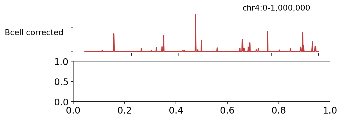
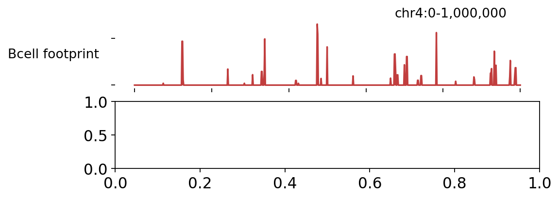
2 · Browse corrected and footprint tracks#
The corrected tracks (top) and the footprint scores (bottom) over a chr4 window — footprint signal peaks where TFs are bound.
bw = ov.epi.bulk.bigwig({'Bcell corrected': str(OUT / 'Bcell_corrected.bw'),
                         'Tcell corrected': str(OUT / 'Tcell_corrected.bw')})
bw.read()
bw.plot_track(chrom='chr4', chromstart=0, chromend=1_000_000,
              color_dict={'Bcell corrected': '#c13e3e', 'Tcell corrected': '#3a6eb3'},
              figwidth=7, figheight=2.5, value_type='max')
plt.show()
└─ Load bigWig files
  ├─ Loading Bcell corrected...
  └─ Loading Tcell corrected...
bw = ov.epi.bulk.bigwig({'Bcell footprint': str(DATA / 'Bcell_footprints.bw'),
                         'Tcell footprint': str(DATA / 'Tcell_footprints.bw')})
bw.read()
bw.plot_track(chrom='chr4', chromstart=0, chromend=1_000_000,
              color_dict={'Bcell footprint': '#c13e3e', 'Tcell footprint': '#3a6eb3'},
              figwidth=7, figheight=2.5, value_type='max')
plt.show()
└─ Load bigWig files
  ├─ Loading Bcell footprint...
  └─ Loading Tcell footprint...
3 · Differential TF binding (BINDetect)#
ov.epi.tl.bindetect scores every JASPAR motif’s footprints in each condition and tests which TFs
change most between B and T cells — the differential-binding workhorse.
ov.epi.tl.bindetect(
    condition_names=['Bcell', 'Tcell'],
    score_files=[str(DATA / 'Bcell_footprints.bw'), str(DATA / 'Tcell_footprints.bw')],
    motif_file=str(DATA / 'motifs.jaspar'), fasta_file=str(DATA / 'genome.fa'),
    regions_bed=str(DATA / 'merged_peaks_annotated.bed'), output_dir=str(OUT / 'bindetect'))

summary = max((OUT / 'bindetect').glob('*_results.txt'), key=lambda p: p.stat().st_size)
tab = pd.read_csv(summary, sep='\t')
cols = [c for c in tab.columns if c in {'output_prefix', 'name', 'motif_id',
        'Bcell_Tcell_change', 'Bcell_Tcell_pvalue'}]
tab[cols].sort_values('Bcell_Tcell_pvalue').head(10)
└─ Starting BINDetect analysis...
└─ Processing input data
└─ Found 6007 regions in input peaks
      └─ Peaks have 8 columns
      └─ Peak header list: ['peak_chr', 'peak_start', 'peak_end', 'additional_1', 'additional_2', 'additional_3', 'additional_4', 'additional_5']
  └─ GC content estimated at 47.61%
  └─ Read 83 motifs
  └─ Plotting sequence logos for each motif
└─ Scanning for motifs and matching to signals...
└─ Processing background scores
└─ Normalizing scores across conditions
└─ Estimating bound/unbound threshold
└─ Threshold estimated at: 10.7384
└─ Calculating differential binding statistics
└─ Processing scanned TFBS individually
└─ Writing results files
└─ Creating plots
└─ BINDetect analysis completed!
| output_prefix | name | motif_id | Bcell_Tcell_change | Bcell_Tcell_pvalue | |
|---|---|---|---|---|---|
| 36 | IRF1_MA0050.2 | IRF1 | MA0050.2 | 0.45392 | 3.672490e-140 |
| 4 | BATF_MA1634.1 | BATF | MA1634.1 | 0.63654 | 1.073840e-133 |
| 38 | JUNB_MA0490.2 | JUNB | MA0490.2 | 0.58744 | 2.038320e-116 |
| 37 | IRF4_MA1419.1 | IRF4 | MA1419.1 | 0.55617 | 3.705740e-116 |
| 57 | NRF1_MA0506.1 | NRF1 | MA0506.1 | -0.36535 | 1.259370e-108 |
| 3 | BACH2_MA1101.2 | BACH2 | MA1101.2 | 0.49062 | 3.812140e-107 |
| 45 | MEF2B_MA0660.1 | MEF2B | MA0660.1 | 0.34917 | 1.765280e-99 |
| 44 | MEF2A_MA0052.4 | MEF2A | MA0052.4 | 0.27290 | 8.179300e-99 |
| 34 | HNF1A_MA0046.2 | HNF1A | MA0046.2 | 0.41346 | 2.565590e-98 |
| 65 | RUNX2_MA0511.2 | RUNX2 | MA0511.2 | 0.32753 | 1.870310e-96 |
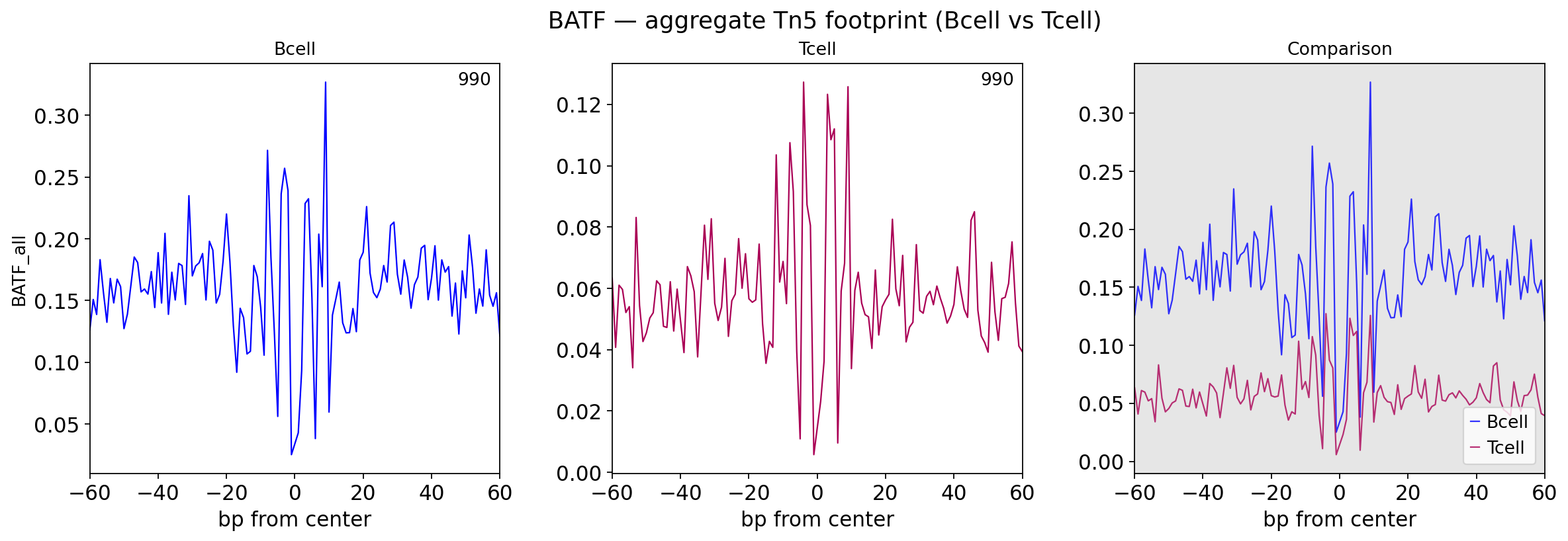
4 · Aggregate footprint at BATF sites#
Averaging the corrected Tn5 signal over all BATF motif sites gives the classic footprint shape — a central dip (TF protection) with flanking accessibility — and its condition difference.
fig = ov.epi.tl.plot_aggregate(
    bigwig_files=[str(OUT / 'Bcell_corrected.bw'), str(OUT / 'Tcell_corrected.bw')],
    regions_bed=str(DATA / 'BATF_all.bed'), output_file=str(OUT / 'BATF_aggregate.pdf'),
    labels=['Bcell', 'Tcell'], title='BATF — aggregate Tn5 footprint (Bcell vs Tcell)')
from IPython.display import display
display(fig)
[PlotAggregate] INFO: ---- Processing input ----
[PlotAggregate] INFO: Reading information from .bed-files
[PlotAggregate] STATS: COUNT BATF_all: 990 sites
[PlotAggregate] INFO: Reading signal from bigwigs
[PlotAggregate] INFO: - Reading signal from Bcell
[PlotAggregate] INFO: - Reading signal from Tcell
[PlotAggregate] INFO: Calculating aggregate signals
[PlotAggregate] INFO: ---- Plotting aggregates ----
[PlotAggregate] INFO: Setting up plotting grid
[PlotAggregate] INFO: Plotting regions BATF_all from signal Bcell
[PlotAggregate] INFO: Plotting regions BATF_all from signal Tcell
[PlotAggregate] INFO: Adjusting final details
[PlotAggregate] INFO: Saved plot to /scratch/users/steorra/analysis/omicverse_dev/guide-upstream-wt/docs/Tutorials-epigenetics/data_epi/footprint/BATF_aggregate.pdf
Summary#
stage |
function |
|---|---|
Tn5 bias correction |
|
browse tracks |
|
differential TF binding |
|
aggregate footprint |
|
Footprinting reads TF occupancy directly off the Tn5 cut pattern — a bulk-ATAC complement to the single-cell chromVAR motif-activity tutorial, and the end of the epigenetics chapter’s tour from reads (ChIP upstream) through 3D genome (Hi-C).