Peptide → protein summarization & the DIA workflow#
A DDA or DIA search engine (MaxQuant, FragPipe, DIA-NN, Spectronaut) does not report protein abundances directly. Its primary output is a long table of feature-level intensities — one row per precursor (peptide + charge) or per fragment ion (peptide + charge + transition), measured in every run. A single protein is observed through many such features, and the number, identity and quality of those features differ from run to run.
Before any differential test you must summarize these features into one number per protein per run. This step is not a formality: it is where most of the systematic bias in a label-free experiment is introduced or removed.
Why a naive mean is wrong:
Outlier features. A mis-identified or interfered transition can be 100× off. On the linear scale a single outlier dominates the mean; even on the log scale it shifts it noticeably.
Missing features. Features drop out non-randomly (low-abundance precursors near the detection limit). A protein quantified by its 3 brightest features in run A and by 8 features including dim ones in run B will look artificially different — a pure feature-composition effect, not biology.
Run effects. Total ion current, LC drift and injection amount vary between runs. These must be modelled per run, not averaged away.
The robust summarizers below all share one idea: model the feature-by-run matrix of one protein as abundance ≈ feature_effect + run_effect, estimate it robustly, and read off the run effects as the protein abundance. This tutorial compares five methods on a real controlled DDA spike-in experiment, then repeats the identical workflow on a real DIA dataset.
Method |
Backend |
Model |
When to use |
|---|---|---|---|
|
|
per-protein median across features |
quick, fully missing-tolerant; ignores feature effects |
|
|
subtract per-feature median, then median across features |
TMT-style; removes feature offsets before collapsing |
|
|
Tukey median polish (robust row+column fit) |
robust to outlier features; DEqMS default |
|
|
Tukey median polish, MSstats formulation |
the MSstats default for DDA/DIA |
|
|
least-squares |
legacy MSstats; sensitive to outliers |
We also run the full MSstats dataProcess pipeline (log-transform + per-run normalization + feature selection + TMP summarization in one call) and finish with differential expression on the summarized protein matrix.
0. Imports#
import omicverse as ov
import pandas as pd
import numpy as np
import anndata as ad
import matplotlib.pyplot as plt

print('core imports ok')
core imports ok
import pymsstats
import pydeqms

ov.plot_set()
print('omicverse', ov.__version__, '| pymsstats', pymsstats.__name__, '| pydeqms', pydeqms.__name__)
🔬 Starting plot initialization...
🧬 Detecting GPU devices…
🚫 No GPU devices found (CUDA/MPS/ROCm/XPU)

   ____            _     _    __
  / __ \____ ___  (_)___| |  / /__  _____________
 / / / / __ `__ \/ / ___/ | / / _ \/ ___/ ___/ _ \
/ /_/ / / / / / / / /__ | |/ /  __/ /  (__  )  __/
\____/_/ /_/ /_/_/\___/ |___/\___/_/  /____/\___/

🔖 Version: 2.2.1rc1   📚 Tutorials: https://omicverse.readthedocs.io/
✅ plot_set complete.

omicverse 2.2.1rc1 | pymsstats pymsstats | pydeqms pydeqms
1. Feature-level DDA data#
ov.datasets.protein_dda_spikein() returns the MSstats DDARawData dataset — a real, controlled label-free DDA spike-in experiment. Six purified proteins were spiked into a constant background at six different concentrations (C1…C6, a dilution series), so the true protein-level fold changes are known by design. Each condition has three technical runs (18 runs total).
The table is in MSstats long format: one row per feature per run, with a fixed, upper-case column schema.
dda = ov.datasets.protein_dda_spikein()
print('shape:', dda.shape)
dda.head()
🔍 Downloading data to ./data/protein_msstats_dda.csv.gz
⚠️ File ./data/protein_msstats_dda.csv.gz already exists
shape: (2070, 10)
| ProteinName | PeptideSequence | PrecursorCharge | FragmentIon | ProductCharge | IsotopeLabelType | Condition | BioReplicate | Run | Intensity | |
|---|---|---|---|---|---|---|---|---|---|---|
| 0 | bovine | S.PVDIDTK_5 | 5 | NaN | NaN | L | C1 | 1 | 1 | 2636791.50 |
| 1 | bovine | S.PVDIDTK_5 | 5 | NaN | NaN | L | C1 | 1 | 2 | 1992418.50 |
| 2 | bovine | S.PVDIDTK_5 | 5 | NaN | NaN | L | C1 | 1 | 3 | 1982146.38 |
| 3 | bovine | S.PVDIDTK_5 | 5 | NaN | NaN | L | C2 | 1 | 4 | 5019594.00 |
| 4 | bovine | S.PVDIDTK_5 | 5 | NaN | NaN | L | C2 | 1 | 5 | 4560467.50 |
# The MSstats long-format schema (column names are exact, upper-case).
for col in dda.columns:
    print(f'{col:18s} {dda[col].dtype}')
ProteinName        object
PeptideSequence    object
PrecursorCharge    int64
FragmentIon        float64
ProductCharge      float64
IsotopeLabelType   object
Condition          object
BioReplicate       int64
Run                int64
Intensity          float64
MSstats long format. Ten columns describe each measurement:
ProteinName— the parent protein (the unit we summarize to).PeptideSequence,PrecursorCharge— together identify a precursor.FragmentIon,ProductCharge— identify a transition (fragment); empty in this DDA table because DDA quantifies at precursor level.IsotopeLabelType—L(light) for a label-free experiment.Condition,BioReplicate,Run— the experimental design.Intensity— the raw linear MS signal (the value we summarize).
A feature is the finest quantified unit. In this DDA table that is ProteinName + PeptideSequence + PrecursorCharge.
n_feat = dda.groupby(['ProteinName', 'PeptideSequence', 'PrecursorCharge']).ngroups
print(f'{dda["ProteinName"].nunique():>4d} proteins')
print(f'{dda["PeptideSequence"].nunique():>4d} peptides')
print(f'{n_feat:>4d} features (peptide + charge)')
print(f'{dda["Run"].nunique():>4d} runs across {dda["Condition"].nunique()} conditions')
6 proteins
 115 peptides
 115 features (peptide + charge)
  18 runs across 6 conditions
# Features per protein, and the experimental design.
print('features per protein:')
print(dda.groupby('ProteinName')['PeptideSequence'].nunique().to_string())
print('\nruns per condition:')
print(dda.groupby('Condition')['Run'].nunique().to_string())
print(f'\nmissing (NaN) intensities: {dda["Intensity"].isna().sum()} / {len(dda)}')
features per protein:
ProteinName
bovine       14
chicken      11
cyc_horse    32
myg_horse    12
rabbit       31
yeast        15

runs per condition:
Condition
C1    3
C2    3
C3    3
C4    3
C5    3
C6    3

missing (NaN) intensities: 698 / 2070
Each protein is seen through 11–32 peptides — so summarization genuinely matters here. About a third of feature×run cells are missing (NaN), exactly the non-random dropout that biases a naive mean. The spike-in design means the six proteins really do change in abundance across the C1…C6 dilution series; a correct summarizer + DE should recover that.
2. Building a peptide-level AnnData#
ov.protein.summarize consumes an AnnData whose X is a runs × features matrix, with var[protein_col] mapping each feature to its parent protein. We build it by pivoting the long table:
rows (
obs) = runs, carrying theConditiondesign,columns (
var) = features, carrying the parentProtein,X= raw linearIntensity(missing features stayNaN).
# A stable feature id: protein | peptide | charge.
dda = dda.copy()
dda['feature'] = (dda['ProteinName'].astype(str) + '|'
                  + dda['PeptideSequence'].astype(str) + '|z'
                  + dda['PrecursorCharge'].astype(str))
wide = dda.pivot_table(index='Run', columns='feature',
                       values='Intensity', aggfunc='first')
print('runs × features:', wide.shape)
runs × features: (18, 115)
# obs = run metadata (Condition group); aligned to the pivot row order.
run_meta = (dda[['Run', 'Condition', 'BioReplicate']]
            .drop_duplicates().set_index('Run').reindex(wide.index))
obs = pd.DataFrame(
    {'Condition': run_meta['Condition'].astype(str).values,
     'BioReplicate': run_meta['BioReplicate'].astype(str).values},
    index=wide.index.astype(str))
obs.head()
| Condition | BioReplicate | |
|---|---|---|
| Run | ||
| 1 | C1 | 1 |
| 2 | C1 | 1 |
| 3 | C1 | 1 |
| 4 | C2 | 1 |
| 5 | C2 | 1 |
# var = feature metadata; the Protein column drives summarization.
feat_meta = (dda[['feature', 'ProteinName', 'PeptideSequence']]
             .drop_duplicates().set_index('feature').reindex(wide.columns))
var = pd.DataFrame(
    {'Protein': feat_meta['ProteinName'].astype(str).values,
     'Peptide': feat_meta['PeptideSequence'].astype(str).values},
    index=wide.columns.astype(str))
var.head()
| Protein | Peptide | |
|---|---|---|
| feature | ||
| bovine|D.GPLTGTYR_23|z23 | bovine | D.GPLTGTYR_23 |
| bovine|F.HFHWGSSDDQGSEHTVDR_402|z402 | bovine | F.HFHWGSSDDQGSEHTVDR_402 |
| bovine|F.HWGSSDDQGSEHTVDR_229|z229 | bovine | F.HWGSSDDQGSEHTVDR_229 |
| bovine|G.PLTGTYR_8|z8 | bovine | G.PLTGTYR_8 |
| bovine|H.SFNVEYDDSQDK_465|z465 | bovine | H.SFNVEYDDSQDK_465 |
pep = ad.AnnData(X=wide.to_numpy(dtype=float), obs=obs, var=var)
pep.uns['source'] = 'MSstats DDARawData (spike-in)'
print(pep)
AnnData object with n_obs × n_vars = 18 × 115
    obs: 'Condition', 'BioReplicate'
    var: 'Protein', 'Peptide'
    uns: 'source'
pep is now a feature-level AnnData: 18 runs × 115 precursor features, with var['Protein'] linking each feature to one of the 6 proteins. This is the standard input to ov.protein.summarize.
3. Summarization methods compared#
ov.protein.summarize(pep, protein_col='Protein', method=...) collapses the 115-feature matrix to a 6-protein matrix. With log2=True (default) the raw linear intensities are log2-transformed first — every summarizer (DEqMS and MSstats) collapses on the log scale, because summarizing raw intensities lets the brightest feature dominate.
We run all five methods and keep each protein-level AnnData.
methods = ['median', 'median_sweeping', 'medpolish', 'tmp', 'linear']
summ = {m: ov.protein.summarize(pep, protein_col='Protein', method=m)
        for m in methods}
for m, a in summ.items():
    print(f'{m:16s} -> {a.shape[0]} runs × {a.shape[1]} proteins   '
          f'(NaN: {int(np.isnan(a.X).sum())})')
median           -> 18 runs × 6 proteins   (NaN: 1)
median_sweeping  -> 18 runs × 6 proteins   (NaN: 1)
medpolish        -> 18 runs × 6 proteins   (NaN: 1)
tmp              -> 18 runs × 6 proteins   (NaN: 0)
linear           -> 18 runs × 6 proteins   (NaN: 1)
Every method returns the same 18 × 6 protein-level matrix — but the values differ. Note the methods produce abundances on different offsets: median/tmp/linear return values near the original log2 scale, while median_sweeping and medpolish return column (run) effects that are centred near zero (each protein’s grand level is removed). That centring is harmless for fold-change — DE works on differences — but means you should never mix summarizers within one analysis.
# How much do methods agree? Correlate the run-by-protein values, flattened.
flat = {m: a.X.ravel() for m, a in summ.items()}
corr = pd.DataFrame(
    {m1: {m2: np.corrcoef(np.vstack([flat[m1], flat[m2]])[:, ~np.isnan(flat[m1])
          & ~np.isnan(flat[m2])])[0, 1]
          for m2 in methods} for m1 in methods})
corr.round(3)
| median | median_sweeping | medpolish | tmp | linear | |
|---|---|---|---|---|---|
| median | 1.000 | 0.731 | 0.711 | 0.806 | 0.837 |
| median_sweeping | 0.731 | 1.000 | 0.972 | 0.939 | 0.933 |
| medpolish | 0.711 | 0.972 | 1.000 | 0.964 | 0.946 |
| tmp | 0.806 | 0.939 | 0.964 | 1.000 | 0.987 |
| linear | 0.837 | 0.933 | 0.946 | 0.987 | 1.000 |
# medpolish vs tmp: both are Tukey median polish, different implementations.
fig, axes = plt.subplots(1, 2, figsize=(9, 4.2))
for ax, (xa, ya) in zip(axes, [('medpolish', 'tmp'), ('median', 'medpolish')]):
    x, y = summ[xa].X.ravel(), summ[ya].X.ravel()
    keep = ~np.isnan(x) & ~np.isnan(y)
    ax.scatter(x[keep], y[keep], s=22, alpha=0.7, edgecolor='none')
    ax.set_xlabel(f'{xa} (log2)'); ax.set_ylabel(f'{ya} (log2)')
    ax.set_title(f'{xa} vs {ya}')
fig.tight_layout(); plt.show()
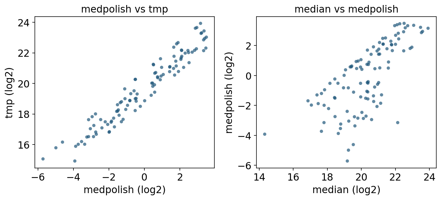
Reading the comparison.
medpolishandtmpare the same algorithm (Tukey median polish) from two backends; they correlate near-perfectly, differing only by the constant per-protein offset (DEqMS keeps column effects, MSstats adds back the protein mean). Either is a sound default.mediandeviates frommedpolishprecisely for proteins with outlier or missing features — the plain median ignores feature effects, so a run that happens to miss the brightest peptides looks lower than it truly is.linearagrees with TMP when features are clean, but its least-squares fit is pulled by outliers, which is why MSstats replaced it with TMP as the default.
Recommendation. Use medpolish / tmp (robust to outlier peptides, missing-tolerant, the MSstats default) for almost every DDA/DIA experiment. median is fine as a fast sanity check or when you have very few peptides per protein. linear is mainly for reproducing legacy MSstats results.
4. The MSstats dataProcess pipeline#
In practice you rarely call a summarizer in isolation. MSstats’ dataProcess bundles the full feature-to-protein preprocessing into one step:
log-transform the raw intensities (
log_base=2),per-run normalization —
equalizeMediansshifts each run so its median log-intensity matches the grand median, removing loading / TIC differences,feature selection — drop features observed in too few runs (
min_feature_obs), which would otherwise inject noise,TMP summarization — collapse the cleaned feature matrix to protein level via Tukey median polish.
pymsstats.data_process takes the MSstats long DataFrame directly — it expects exactly the upper-case schema (ProteinName, PeptideSequence, PrecursorCharge, FragmentIon, ProductCharge, IsotopeLabelType, Condition, BioReplicate, Run, Intensity), which the ov.datasets loader already provides, so no renaming is needed.
import inspect
print('data_process signature:')
print(' ', inspect.signature(pymsstats.data_process))
print('\nrequired columns (pymsstats.CANONICAL_COLS):')
print(' ', pymsstats.CANONICAL_COLS)
print('\nDDA table matches schema:',
      set(pymsstats.CANONICAL_COLS).issubset(dda.columns))
data_process signature:
  (msstats_df: 'pd.DataFrame', *, normalization: 'str' = 'equalizeMedians', summary_method: 'str' = 'TMP', log_base: 'int' = 2, min_feature_obs: 'int' = 2, censored_int: 'str' = 'NA') -> 'pd.DataFrame'

required columns (pymsstats.CANONICAL_COLS):
  ['ProteinName', 'PeptideSequence', 'PrecursorCharge', 'FragmentIon', 'ProductCharge', 'IsotopeLabelType', 'Condition', 'BioReplicate', 'Run', 'Intensity']

DDA table matches schema: True
# Full MSstats preprocessing: log2 + equalizeMedians + feature select + TMP.
msstats_cols = list(pymsstats.CANONICAL_COLS)
processed = pymsstats.data_process(
    dda[msstats_cols],
    normalization='equalizeMedians',
    summary_method='TMP',
    log_base=2,
    min_feature_obs=2,
)
print('processed shape:', processed.shape)
processed.head()
processed shape: (108, 7)
| Protein | RUN | LogIntensities | n_features | n_obs | GROUP | SUBJECT | |
|---|---|---|---|---|---|---|---|
| 0 | bovine | 1 | 21.349305 | 14 | 164 | C1 | 1 |
| 1 | bovine | 10 | 17.426372 | 14 | 164 | C4 | 1 |
| 2 | bovine | 11 | 17.406355 | 14 | 164 | C4 | 1 |
| 3 | bovine | 12 | 16.390505 | 14 | 164 | C4 | 1 |
| 4 | bovine | 13 | 18.490566 | 14 | 164 | C5 | 1 |
data_process returns a long protein-level table: one row per Protein × RUN, with LogIntensities (the summarized protein abundance), n_features / n_obs (how many features and observations fed each protein), and the design columns GROUP / SUBJECT. 6 proteins × 18 runs = 108 rows.
We pivot it into the same runs × proteins AnnData shape used above, so it can flow into ov.protein.de exactly like the summarize output.
wide_proc = processed.pivot_table(index='RUN', columns='Protein',
                                  values='LogIntensities', aggfunc='first')
proc_obs = (processed[['RUN', 'GROUP', 'SUBJECT']].drop_duplicates()
            .set_index('RUN').reindex(wide_proc.index))
dp_adata = ad.AnnData(
    X=wide_proc.to_numpy(dtype=float),
    obs=pd.DataFrame({'Condition': proc_obs['GROUP'].astype(str).values},
                     index=wide_proc.index.astype(str)),
    var=pd.DataFrame(index=wide_proc.columns.astype(str)))
print('MSstats dataProcess -> protein AnnData:', dp_adata.shape)
print(dp_adata.obs['Condition'].value_counts().to_string())
MSstats dataProcess -> protein AnnData: (18, 6)
Condition
C1    3
C4    3
C5    3
C6    3
C2    3
C3    3
dataProcess and ov.protein.summarize(method='tmp') use the same TMP core; dataProcess additionally normalizes per run and applies feature filtering, so it is the recommended one-call route for a real MSstats DDA/DIA experiment. ov.protein.summarize exposes the individual summarizers so you can compare them — as we did in Section 3.
5. Differential expression on the summarized matrix#
Summarization produced a protein-level matrix on the log2 scale — exactly the input ov.protein.de expects. We take the medpolish-summarized AnnData and test one contrast of the spike-in dilution series.
We pick C2 vs C5, two well-separated dilution levels. Because the six proteins were spiked at different concentrations per condition, a correct summarize → DE pipeline should flag them as differential, with signed fold changes that track the dilution direction.
prot = summ['medpolish']
contrast = prot[prot.obs['Condition'].isin(['C2', 'C5'])].copy()
print('contrast subset:', contrast.shape)
print(contrast.obs['Condition'].value_counts().to_string())
contrast subset: (6, 6)
Condition
C2    3
C5    3
de_dda = ov.protein.de(contrast, group='Condition',
                       method='limma', reference='C2')
de_dda
| gene | logFC | AveExpr | t | P.Value | adj.P.Val | |
|---|---|---|---|---|---|---|
| 0 | chicken | -3.992743 | -1.180237 | -14.499797 | 1.215084e-47 | 7.290506e-47 |
| 1 | bovine | -3.753528 | 1.224481 | -13.631077 | 2.616879e-42 | 7.850637e-42 |
| 2 | yeast | 3.704893 | 1.138670 | 13.454457 | 2.898620e-41 | 5.797240e-41 |
| 3 | myg_horse | 3.624045 | -1.171078 | 13.160856 | 1.474069e-39 | 2.211104e-39 |
| 4 | cyc_horse | -3.340364 | 0.279009 | -12.130656 | 7.266499e-34 | 8.719799e-34 |
| 5 | rabbit | 3.271494 | -0.095772 | 11.880553 | 1.493758e-32 | 1.493758e-32 |
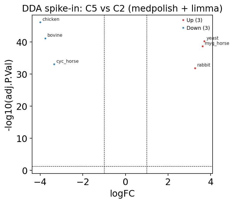
limma (Smyth 2004 empirical-Bayes moderated t) is appropriate here: with only 3 runs per condition, borrowing variance information across proteins stabilizes the per-protein test. The logFC column is C5 - C2 on the log2 scale. With a controlled spike-in, all six proteins are expected to move — the table confirms the summarized matrix carries real, separable signal.
ov.protein.volcano(de_dda, logfc_threshold=1.0, adj_p_threshold=0.05,
                   title='DDA spike-in: C5 vs C2 (medpolish + limma)')
plt.show()
# Does the summarizer choice change the DE call? Re-run on the TMP matrix.
tmp_contrast = summ['tmp'][summ['tmp'].obs['Condition'].isin(['C2', 'C5'])].copy()
de_tmp = ov.protein.de(tmp_contrast, group='Condition',
                       method='limma', reference='C2')
cmp = (de_dda.set_index('gene')[['logFC', 'adj.P.Val']]
       .join(de_tmp.set_index('gene')[['logFC', 'adj.P.Val']],
             lsuffix='_medpolish', rsuffix='_tmp'))
cmp.round(3)
| logFC_medpolish | adj.P.Val_medpolish | logFC_tmp | adj.P.Val_tmp | |
|---|---|---|---|---|
| gene | ||||
| chicken | -3.993 | 0.0 | -3.862 | 0.0 |
| bovine | -3.754 | 0.0 | -3.818 | 0.0 |
| yeast | 3.705 | 0.0 | 3.678 | 0.0 |
| myg_horse | 3.624 | 0.0 | 3.587 | 0.0 |
| cyc_horse | -3.340 | 0.0 | -3.324 | 0.0 |
| rabbit | 3.271 | 0.0 | 3.231 | 0.0 |
The two robust summarizers give near-identical fold changes and significance — reassuring: when the summarizer is robust, the downstream DE is stable. The summarizer choice would matter much more on a noisier, missing-value-heavy dataset, which is exactly why the robust medpolish/tmp methods are the default.
6. The DIA workflow#
ov.datasets.protein_dia() returns the MSstats DIARawData dataset — a real label-free DIA experiment comparing Streptococcus pyogenes grown at two serum concentrations (Strep 0% vs Strep 10%), 2 biological replicates each.
How DIA differs from DDA. In DDA the instrument picks individual precursors to fragment, so quantification is sparse and stochastic — a precursor missed in one run is simply absent. DIA fragments all precursors in wide isolation windows every cycle, giving deeper, more reproducible, more complete quantification. The flip side: DIA spectra are chimeric, so quantification is done at the fragment-ion (transition) level — the FragmentIon and ProductCharge columns are now populated, and the feature is peptide + charge + fragment + product-charge.
Crucially, the ov.protein workflow is identical: the same MSstats long schema, the same summarize → de path.
dia = ov.datasets.protein_dia()
print('shape:', dia.shape)
print('proteins:', dia['ProteinName'].nunique(),
      '| peptides:', dia['PeptideSequence'].nunique(),
      '| runs:', dia['Run'].nunique())
dia.head()
🔍 Downloading data to ./data/protein_msstats_dia.csv.gz
⚠️ File ./data/protein_msstats_dia.csv.gz already exists
shape: (980, 10)
proteins: 2 | peptides: 32 | runs: 4
| ProteinName | PeptideSequence | PrecursorCharge | FragmentIon | ProductCharge | IsotopeLabelType | Condition | BioReplicate | Run | Intensity | |
|---|---|---|---|---|---|---|---|---|---|---|
| 0 | RNA helicase exp9 | ASPIQEMTIPLALEGK | 2 | b9 | 77414 | L | Strep 0% | 1 | 1 | 9747 |
| 1 | RNA helicase exp9 | ASPIQEMTIPLALEGK | 2 | y10 | 77411 | L | Strep 0% | 1 | 1 | 1272 |
| 2 | RNA helicase exp9 | ASPIQEMTIPLALEGK | 2 | y11 | 77412 | L | Strep 0% | 1 | 1 | 1295 |
| 3 | RNA helicase exp9 | ASPIQEMTIPLALEGK | 2 | y14 | 77410 | L | Strep 0% | 1 | 1 | 2332 |
| 4 | RNA helicase exp9 | ASPIQEMTIPLALEGK | 2 | y7 | 77409 | L | Strep 0% | 1 | 1 | 8178 |
# DIA design: 2 conditions x 2 biological replicates.
print(dia[['Run', 'Condition', 'BioReplicate']].drop_duplicates().to_string(index=False))
n_dia_feat = dia.groupby(['ProteinName', 'PeptideSequence', 'PrecursorCharge',
                          'FragmentIon', 'ProductCharge']).ngroups
print(f'\nfragment-level features: {n_dia_feat}')
Run Condition  BioReplicate
   1  Strep 0%             1
   2  Strep 0%             2
   3 Strep 10%             1
   4 Strep 10%             2

fragment-level features: 245
# Build a fragment-level AnnData: feature = peptide|charge|fragment|prodcharge.
dia = dia.copy()
dia['feature'] = (dia['PeptideSequence'].astype(str) + '|z'
                  + dia['PrecursorCharge'].astype(str) + '|'
                  + dia['FragmentIon'].astype(str) + '|'
                  + dia['ProductCharge'].astype(str))
dia_wide = dia.pivot_table(index='Run', columns='feature',
                           values='Intensity', aggfunc='first')
print('runs × fragment features:', dia_wide.shape)
runs × fragment features: (4, 245)
dia_runmeta = (dia[['Run', 'Condition', 'BioReplicate']]
               .drop_duplicates().set_index('Run').reindex(dia_wide.index))
dia_featmap = (dia[['feature', 'ProteinName']]
               .drop_duplicates().set_index('feature').reindex(dia_wide.columns))
dia_pep = ad.AnnData(
    X=dia_wide.to_numpy(dtype=float),
    obs=pd.DataFrame({'Condition': dia_runmeta['Condition'].astype(str).values},
                     index=dia_wide.index.astype(str)),
    var=pd.DataFrame({'Protein': dia_featmap['ProteinName'].astype(str).values},
                     index=dia_wide.columns.astype(str)))
dia_pep.uns['source'] = 'MSstats DIARawData (S. pyogenes)'
print(dia_pep)
AnnData object with n_obs × n_vars = 4 × 245
    obs: 'Condition'
    var: 'Protein'
    uns: 'source'
# Identical summarize step — collapse 245 fragments to 2 proteins via TMP.
dia_prot = ov.protein.summarize(dia_pep, protein_col='Protein', method='medpolish')
print('DIA protein-level:', dia_prot.shape)
print(pd.DataFrame(dia_prot.X, index=dia_prot.obs_names,
                   columns=dia_prot.var_names).round(3))
DIA protein-level: (4, 2)
protein   FabG  RNA  helicase exp9
Run
1        0.882              -0.136
2        0.935               0.130
3       -0.871              -0.308
4       -1.244               0.218
# Identical DE step — Strep 10% vs Strep 0%.
de_dia = ov.protein.de(dia_prot, group='Condition',
                       method='limma', reference='Strep 0%')
de_dia
| gene | logFC | AveExpr | t | P.Value | adj.P.Val | |
|---|---|---|---|---|---|---|
| 0 | FabG | -1.965724 | -0.074792 | -7.948313 | 1.890689e-15 | 3.781377e-15 |
| 1 | RNA helicase exp9 | -0.042263 | -0.023843 | -0.170887 | 8.643128e-01 | 8.643128e-01 |
# Cross-check with the MSstats dataProcess route on the same DIA data.
dia_processed = pymsstats.data_process(
    dia[list(pymsstats.CANONICAL_COLS)],
    normalization='equalizeMedians', summary_method='TMP', log_base=2)
print('dataProcess DIA output:', dia_processed.shape)
dia_processed[['Protein', 'RUN', 'LogIntensities', 'GROUP']].head(8)
dataProcess DIA output: (8, 7)
| Protein | RUN | LogIntensities | GROUP | |
|---|---|---|---|---|
| 0 | RNA helicase exp9 | 1 | 10.971460 | Strep 0% |
| 1 | RNA helicase exp9 | 2 | 11.102063 | Strep 0% |
| 2 | RNA helicase exp9 | 3 | 11.450784 | Strep 10% |
| 3 | RNA helicase exp9 | 4 | 11.934159 | Strep 10% |
| 4 | FabG | 1 | 12.446578 | Strep 0% |
| 5 | FabG | 2 | 12.365709 | Strep 0% |
| 6 | FabG | 3 | 11.327864 | Strep 10% |
| 7 | FabG | 4 | 10.944582 | Strep 10% |
Two proteins, two conditions: FabG shows a clear, significant abundance change between the serum conditions while the RNA helicase does not — the expected biological contrast. The point of this section is the method invariance: DDA precursor-level data and DIA fragment-level data flow through the same summarize → de (or dataProcess) code with nothing changed but how the feature id is constructed.
Summary#
The peptide → protein step is mandatory. Search engines emit feature-level (precursor or fragment) intensities; differential testing needs a protein-level matrix. Skipping summarization — or doing it with a naive mean — lets outlier features, non-random missingness and run effects masquerade as biology.
Which summarizer.
medpolish/tmp(Tukey median polish) — default choice. Robust to outlier peptides, missing-tolerant, models feature + run effects jointly. The MSstats default.median— fast, fully missing-tolerant, but ignores feature effects; good as a sanity check or when peptides per protein are very few.median_sweeping— removes per-feature offsets before collapsing (TMT-style); returns centred run effects.linear— least-squaresRUN + FEATURE; reproduces legacy MSstats but is outlier-sensitive.
Two routes in omicverse:
ov.protein.summarize(pep_adata, method=...)— a single summarizer on a feature-level AnnData; use it to compare methods.pymsstats.data_process(long_df, ...)— the full MSstats pipeline (log + per-run normalization + feature filtering + TMP) in one call; the recommended production route for a real DDA/DIA experiment.
DDA vs DIA. DIA quantifies at the fragment level and is deeper / more complete, but the omicverse workflow is identical — the same MSstats long schema, the same summarize → de path.
Next steps.
Bulk LC-MS/MS best-practice pipeline — the complete protein-level workflow (QC → imputation → DE → enrichment).
Missing values: diagnosis & imputation — handling the non-random dropout seen here.
Differential expression: methods compared — DEqMS vs proDA vs MSstats vs limma, contrasts and power.