Bulk LC-MS/MS proteomics — the best-practice pipeline

This is the flagship ov.protein tutorial. It walks the complete, statistically defensible workflow for a bulk label-free quantification (LFQ) proteomics experiment, on a real published dataset, and — just as importantly — explains why each step is done the way it is.

Why proteomics is not RNA-seq

If you bring an RNA-seq mindset to a protein-intensity matrix you will get the wrong answer. Three structural differences drive everything in this tutorial:

1. Missing values are informative, not random. In RNA-seq a zero count is still a measurement. In LC-MS/MS a missing value usually means the peptide signal fell below the instrument’s detection limit — the protein was there, just too low to be sampled by the mass spectrometer. This is left-censored, missing-not-at-random (MNAR) missingness. Naively dropping or mean-imputing these values biases low-abundance proteins toward looking more abundant than they are, and silently destroys real biology. Diagnosing the missingness mechanism before touching it is the single most important habit in proteomics.

2. Per-run sample loading differs. Each LC-MS/MS injection loads a slightly different total amount of protein and the instrument response drifts. Raw intensities therefore carry a multiplicative per-sample offset that has nothing to do with biology. This must be removed by normalization (median / quantile alignment) before any sample-to-sample comparison — the analogue of library-size normalization, but the offsets are larger and noisier.

3. Protein-level variance depends on how many peptides built the protein. A protein quantified from 12 peptides is far more precise than one quantified from a single peptide. Modern moderated tests (DEqMS) use the peptide count as a variance prior. This dataset is a finished protein-intensity matrix with no peptide-count column, so we cannot use that prior here — peptide-count-aware DE is the subject of tutorial 4. Here we instead use proDA, whose probabilistic dropout model is the right tool for genuinely MNAR data.

The pipeline

load → QC → missing-value diagnosis → MCAR/MNAR classification
     → normalize → informed imputation → differential expression
     → volcano / heatmap → functional enrichment

Every stage below is one ov.protein dispatcher call with a method= selector — the same design as ov.es and ov.metabol.

0. Setup

ov.protein is AnnData-native: samples are rows (obs), proteins are columns (var), and adata.X holds the intensity matrix (with NaN for missing values).

import omicverse as ov
import numpy as np
import pandas as pd
import matplotlib.pyplot as plt
ov.plot_set()

🔬 Starting plot initialization...
🧬 Detecting GPU devices…
🚫 No GPU devices found (CUDA/MPS/ROCm/XPU)

   ____            _     _    __                  
  / __ \____ ___  (_)___| |  / /__  _____________ 
 / / / / __ `__ \/ / ___/ | / / _ \/ ___/ ___/ _ \ 
/ /_/ / / / / / / / /__ | |/ /  __/ /  (__  )  __/ 
\____/_/ /_/ /_/_/\___/ |___/\___/_/  /____/\___/                                              

🔖 Version: 2.2.1rc1   📚 Tutorials: https://omicverse.readthedocs.io/
✅ plot_set complete.

1. Load the data

We use ProteomeXchange PXD000022 — a real, published label-free LFQ study comparing two conditions, MB and MT, with three biological replicates each. It is a protein-level intensity matrix: 660 proteins × 6 samples.

In a real project you would not download a pre-built matrix — you would parse your search-engine output with the matching ov.protein reader:

Search engine	Reader
MaxQuant (proteinGroups.txt)	ov.protein.read_maxquant(...)
DIA-NN (report.tsv / pg_matrix)	ov.protein.read_diann(...)
FragPipe (combined_protein.tsv)	ov.protein.read_fragpipe(...)
Olink NPX	ov.protein.read_olink_npx(...)

All readers return the same AnnData layout, so the rest of this pipeline is identical regardless of upstream software.

adata = ov.datasets.protein_pxd000022()
X = np.asarray(adata.X, dtype=float)
overall_missing = 100.0 * np.isnan(X).mean()
print(f"matrix: {adata.shape[0]} samples × {adata.shape[1]} proteins")
print(f"groups: {adata.obs['group'].value_counts().to_dict()}")
print(f"overall missing: {overall_missing:.1f}%")

🔍 Downloading data to ./data/protein_pxd000022.h5ad
⚠️ File ./data/protein_pxd000022.h5ad already exists
matrix: 6 samples × 660 proteins
groups: {'MB': 3, 'MT': 3}
overall missing: 39.9%

~40% of the matrix is missing. That is entirely typical for label-free DDA proteomics and is not a data-quality problem — it is the physics of the instrument. The whole tutorial is built around handling it correctly rather than pretending it away.

2. Quality control

QC removes proteins that are too sparsely observed to be analysed reliably. ov.protein.qc_filter applies two filters:

• min_peptides — drops proteins quantified from too few peptides (low-confidence identifications). This dataset has no peptides column, so this filter is auto-skipped — qc_filter detects the missing column and reports it.

• min_valid — drops proteins observed (non-NaN) in fewer than this fraction of samples. A protein seen in only 1 of 6 samples cannot support a two-group comparison; min_valid=0.5 keeps proteins measured in at least half the samples.

Filtering before diagnosing missingness is correct: we only want the missingness mechanism of proteins we will actually test.

n_before = adata.n_vars
ov.protein.qc_filter(adata, min_peptides=2, min_valid=0.5)
print(f"proteins before QC: {n_before}")
print(f"proteins after  QC: {adata.n_vars}  ({n_before - adata.n_vars} removed)")

proteins before QC: 660
proteins after  QC: 458  (202 removed)

ov.protein.boxplot(adata, color_by='group')
plt.suptitle('Raw intensities — note the per-sample median shifts', y=1.02)
plt.show()

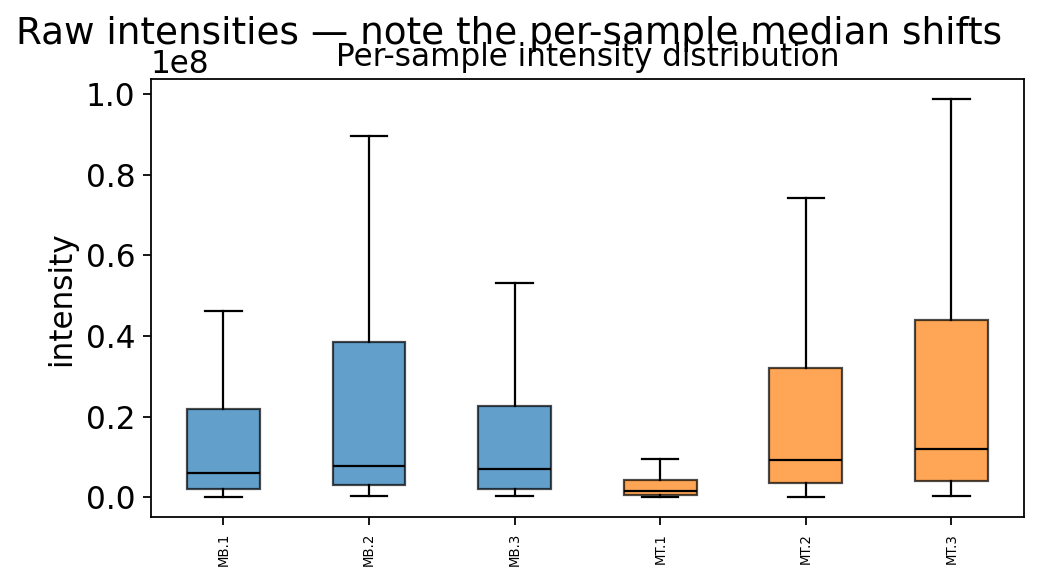
The boxplots above are of raw, un-normalized intensities. The sample medians do not line up — each LC-MS/MS run loaded a slightly different amount of material. Comparing groups on this data directly would confound biology with loading. We fix it in step 4, but first we must understand the missing values.

3. Missing-value diagnostics — the heart of proteomics QC

Before imputing anything, you must answer one question: why are the values missing? There are two mechanisms, and they demand opposite treatments:

• MCAR (missing completely at random) — a value is missing for reasons unrelated to its true abundance (a stochastic acquisition glitch, an integration failure). MCAR values can be imputed with neighbour-based methods (KNN, SVD) that borrow from co-varying proteins.

• MNAR (missing not at random) — a value is missing because it is low: the peptide signal sat below the detection limit. MNAR values must be imputed with left-censored methods that place the imputed value down in the low tail (MinDet, MinProb, QRILC).

Use a KNN imputer on MNAR data and you fill genuine low-abundance holes with mid-range neighbour values — inflating those proteins and erasing the very signal you came to find. So we diagnose first.

mp = ov.protein.missing_pattern(adata)
print(f"overall missing fraction : {mp['overall']:.3f}")
print(f"per-sample missing range : "
      f"{np.min(mp['sample_missing_frac']):.3f} – {np.max(mp['sample_missing_frac']):.3f}")
fully_obs = int(np.sum(np.asarray(mp['protein_missing_frac']) == 0.0))
print(f"proteins with zero missing values: {fully_obs} / {adata.n_vars}")

overall missing fraction : 0.259
per-sample missing range : 0.114 – 0.568
proteins with zero missing values: 113 / 458

ov.protein.missing_pattern_plot(adata, max_proteins=458)
plt.show()

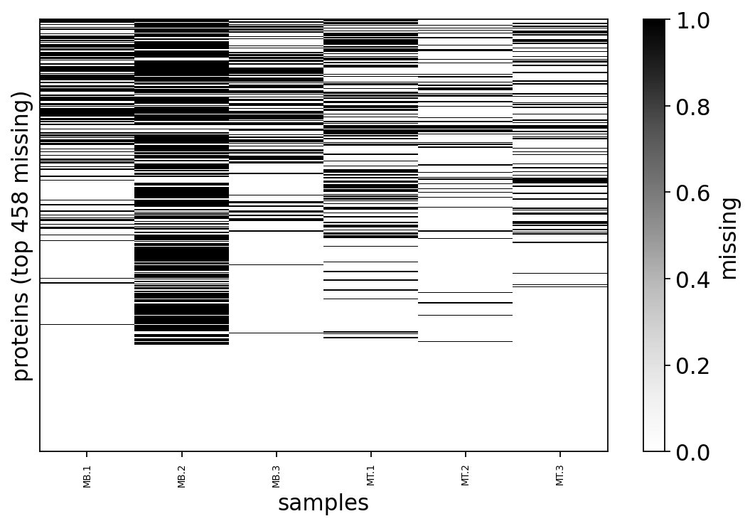
The missingness map above shows missing values are structured, not scattered uniformly — whole blocks of proteins are absent from particular samples. Structure is the first fingerprint of MNAR. To confirm it we look directly at the relationship between a protein’s abundance and its chance of being missing: if low-abundance proteins are missing more often, the missingness is being driven by abundance, i.e. it is MNAR.

Xq = np.asarray(adata.X, dtype=float)
mean_obs = np.nanmean(np.log2(Xq), axis=0)
miss_frac = np.isnan(Xq).mean(axis=0)
ok = np.isfinite(mean_obs)
rho = np.corrcoef(mean_obs[ok], miss_frac[ok])[0, 1]
print(f"corr(mean log2 abundance, missing fraction) = {rho:.3f}")

corr(mean log2 abundance, missing fraction) = -0.555

fig, ax = plt.subplots(figsize=(5.4, 4.2))
ax.scatter(mean_obs[ok], miss_frac[ok], s=14, alpha=0.5, color='#1f77b4')
ax.set_xlabel('mean observed log2 intensity')
ax.set_ylabel('fraction of samples missing')
ax.set_title(f'Low-abundance proteins go missing more often  (r = {rho:.2f})')
plt.show()

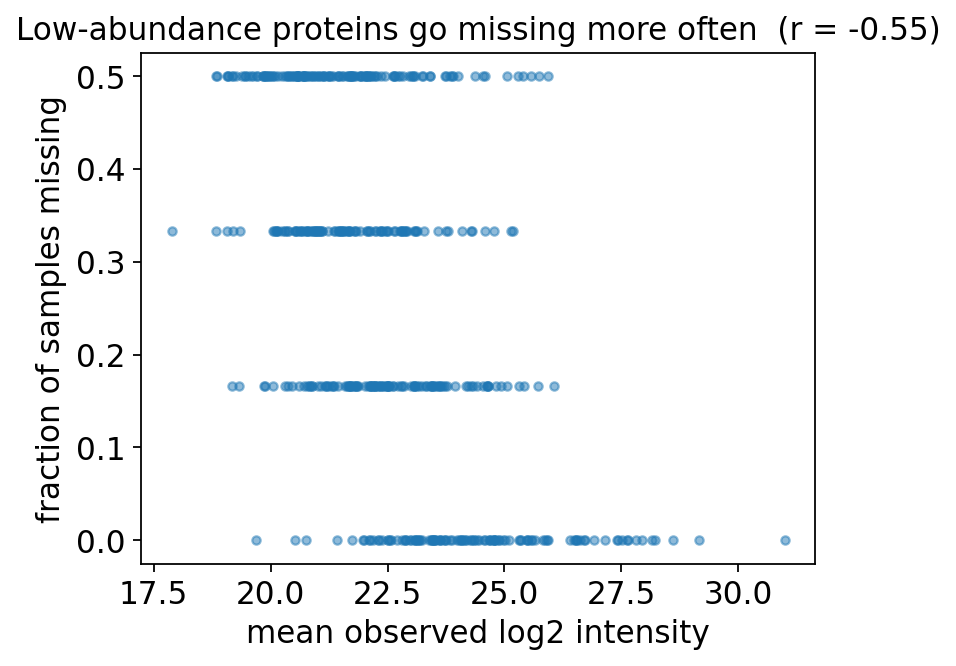
The scatter has a clear downward slope: the dimmer a protein, the more often it is missing. That negative correlation is the signature of left-censored MNAR missingness — exactly what LC-MS/MS physics predicts. This finding dictates our imputer choice in step 5.

ov.protein.model_selector formalises this per protein. It compares each protein’s observed values against an estimated detection threshold and labels it MCAR or MNAR, writing the verdict to adata.var['is_mcar']. Proteins whose missing values sit far below their observed values are MNAR; the rest are treated as MCAR. The returned threshold is the estimated global censoring boundary.

# model_selector compares observed values to an estimated detection
# threshold; run it on a log2 copy so the threshold is on the abundance scale.
adata_log = adata.copy()
adata_log.X = np.log2(np.asarray(adata.X, dtype=float))
mcar_mask, threshold = ov.protein.model_selector(adata_log)
n_mcar = int(np.sum(mcar_mask))
n_mnar = int(adata.n_vars - n_mcar)
adata.var['is_mcar'] = adata_log.var['is_mcar'].to_numpy()
print(f"estimated detection threshold (log2): {threshold:.2f}")
print(f"MCAR-classified proteins      : {n_mcar}")
print(f"MNAR-classified proteins      : {n_mnar}")

estimated detection threshold (log2): 18.83
MCAR-classified proteins      : 456
MNAR-classified proteins      : 2

Read this together with the scatter, not in isolation. model_selector flags an individual protein as MNAR only when its specific missing values demonstrably sit at the low extreme of the abundance distribution; with just 6 samples per protein that per-protein test has very little statistical power, so most proteins fall into the MCAR bucket by default. The population-level abundance-missingness correlation computed above (r ≈ -0.55) is far stronger evidence — and it says the dataset as a whole is dominated by left-censored missingness.

When the per-protein and population views disagree on a small dataset, trust the population view: we treat PXD000022 as MNAR and choose a left-censored imputer accordingly in step 5. model_selector still earns its keep — it writes a per-protein adata.var['is_mcar'] flag that downstream tools (and the method='auto' imputer) can use to handle the handful of genuinely-MCAR proteins differently.

4. Normalization

Now we remove the per-run loading differences seen in the step-2 boxplots. ov.protein.normalize offers several method= options:

• median — shift every sample so its median matches the global median. Robust, assumption-light, the safe default.

• quantile — force every sample to share an identical intensity distribution. Stronger, but assumes the distributions should be identical.

• equalize_medians / log2 — finer-grained variants.

We use median normalization with log2=True. The log2 transform is essential: intensities span ~6 orders of magnitude and are multiplicatively noisy; on the log scale the noise becomes roughly additive and homoscedastic, which is what every downstream linear model assumes. We do this after the missingness diagnosis so the diagnosis reflects the raw acquisition, not a transformed view.

ov.protein.normalize(adata, method='median', log2=True)
print(f"normalized + log2-transformed; X range: "
      f"{np.nanmin(adata.X):.1f} – {np.nanmax(adata.X):.1f}")

normalized + log2-transformed; X range: 16.3 – 33.5

ov.protein.boxplot(adata, color_by='group')
plt.suptitle('After median normalization — sample medians now aligned', y=1.02)
plt.show()

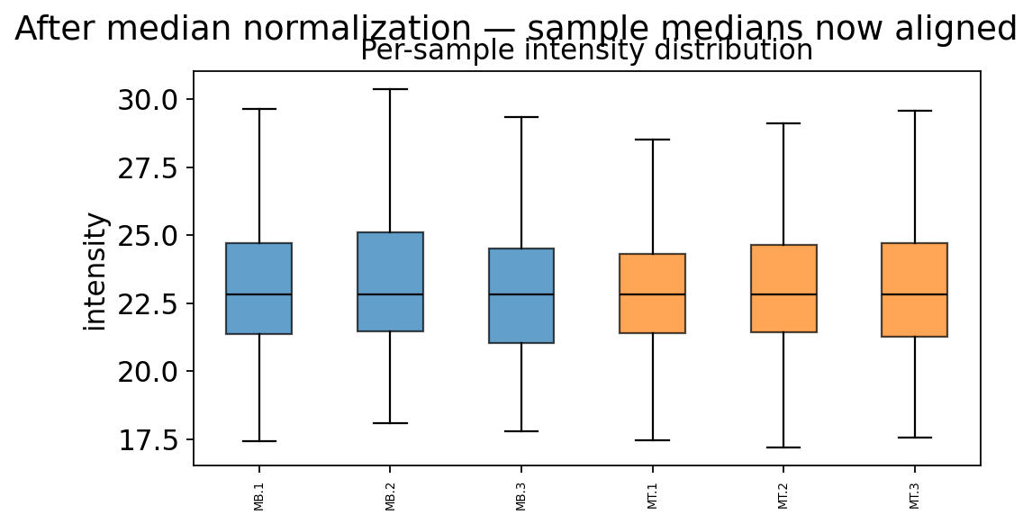
The sample medians now sit on one line. Any remaining between-sample difference is biology (or noise), not loading. We are ready to deal with the holes.

5. Informed imputation

Step 3 told us the missingness is MNAR / left-censored. The imputer must therefore place imputed values down in the low tail, where the true (undetected) abundances actually live. To make the consequences concrete we compare three imputers before committing:

• mindet — deterministic minimum: fills each missing value near the lowest observed intensity. Left-censored. ✓

• qrilc — Quantile Regression Imputation of Left-Censored data: draws imputed values from a truncated Gaussian fitted to the left tail of the distribution. Left-censored, and (unlike mindet) preserves realistic variance. ✓

• knn — k-nearest-neighbour: fills a hole with the average of co-varying proteins. Designed for MCAR — it places values in the middle of the observed range. ✗ for MNAR.

We overlay the imputed-value distributions on the observed distribution. A correct MNAR imputer’s values should sit to the left of the observed mass.

obs_vals = np.asarray(adata.X, dtype=float)
miss = np.isnan(obs_vals)
imputed = {}
for m in ['mindet', 'qrilc', 'knn']:
    tmp = adata.copy()
    ov.protein.impute(tmp, method=m, seed=0)
    imputed[m] = np.asarray(tmp.X, dtype=float)[miss]

fig, ax = plt.subplots(figsize=(6.4, 4.2))
bins = np.linspace(np.nanmin(obs_vals), np.nanmax(obs_vals), 45)
ax.hist(obs_vals[~miss], bins=bins, density=True, color='0.6',
        alpha=0.55, label='observed')
for m, c in zip(['mindet', 'qrilc', 'knn'], ['#2ca02c', '#1f77b4', '#d62728']):
    ax.hist(imputed[m], bins=bins, density=True, histtype='step',
            lw=2, color=c, label=f'imputed: {m}')
ax.set_xlabel('log2 intensity'); ax.set_ylabel('density'); ax.legend()
ax.set_title('Where each imputer places the missing values')
plt.show()

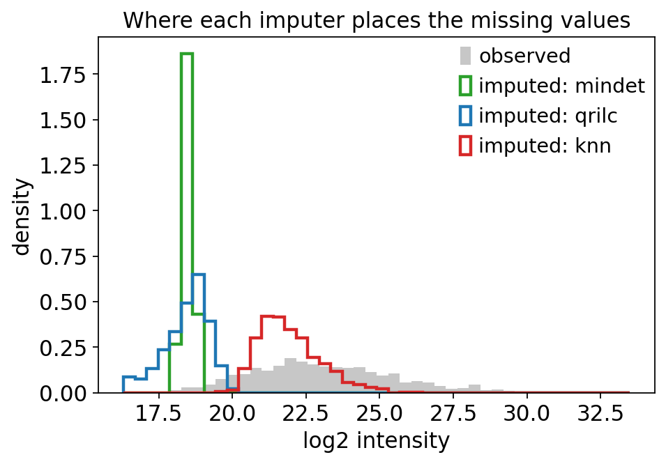
The histogram makes the choice unambiguous. mindet and qrilc put their imputed values in the low tail, below the bulk of the observed data — consistent with values that were missing because they were below detection. knn instead drops its imputed values right in the middle of the observed range: it has invented mid-abundance measurements for proteins that were in fact too dim to detect. On this MNAR dataset knn would systematically inflate low-abundance proteins and manufacture false differential expression.

We commit to qrilc: it is left-censored and stochastic, so it restores realistic per-protein variance instead of collapsing every hole onto a single value (which would understate uncertainty and produce over-confident p-values). seed=0 makes the draw reproducible.

ov.protein.impute(adata, method='qrilc', seed=0)
print(f"missing values remaining: {int(np.isnan(adata.X).sum())}")
print(f"imputed matrix range: {adata.X.min():.1f} – {adata.X.max():.1f}")

missing values remaining: 0
imputed matrix range: 11.2 – 33.5

ov.protein.pca_plot(adata, color='group')
plt.show()

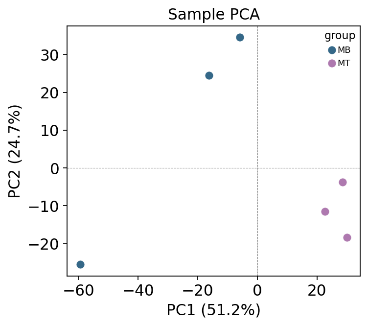
After a correct pipeline — QC, normalization, MNAR-aware imputation — the two groups separate cleanly on PC1. This is the sanity check that the preprocessing recovered biological structure rather than smearing it. If the groups did not separate here, you would revisit the upstream steps before trusting any differential expression.

6. Differential expression

ov.protein.de dispatches several method= engines. Choosing the right one matters:

• proda — a probabilistic model (the proDA package) that explicitly models the dropout curve: it does not need values imputed, because it treats a missing value as evidence that the protein lies below the detection limit and integrates over that uncertainty. For a genuinely MNAR dataset like this one, that is the principled choice — it uses the missing values as information instead of throwing a guess at them.

• limma — empirical-Bayes moderated t-test. Industry standard, but it needs a complete matrix, so it runs on the imputed data and is therefore at the mercy of the imputer.

• welch_t — a plain per-protein Welch t-test. No variance sharing across proteins; with only 3 vs 3 replicates it is badly underpowered — included as a baseline to show what not to rely on.

• deqms — the peptide-count-aware moderated test; not applicable here (no peptide counts) and the focus of tutorial 4.

We run proda on the normalized but un-imputed matrix — letting it see the missing values — then compare against limma and welch_t. reference='MB' makes MB the baseline, so a positive logFC means higher in MT.

# proDA models dropout directly: feed it the normalized but UN-imputed matrix.
# ov.protein.impute kept the pre-imputation values in the 'pre_impute' layer.
adata_mnar = adata.copy()
adata_mnar.X = np.asarray(adata_mnar.layers['pre_impute'], dtype=float)
res = ov.protein.de(adata_mnar, group='group', method='proda', reference='MB')
print(f"proDA: {len(res)} proteins tested  ({int(np.isnan(adata_mnar.X).sum())} NaNs as dropout)")
res.head()

proDA: 458 proteins tested  (711 NaNs as dropout)

	gene	P.Value	adj.P.Val	logFC	t	se	df	AveExpr	n_obs
0	F1MXE4	0.000018	0.007245	-3.120031	-23.921306	0.130429	4.0	20.936220	3
1	O08532-2	0.000064	0.012828	3.499900	17.393134	0.201223	4.0	24.123182	5
2	F6QX36	0.000141	0.018815	1.135398	14.243413	0.079714	4.0	23.926828	3
3	F6ZJB0	0.000237	0.023681	-2.978078	-12.483926	0.238553	4.0	22.659999	3
4	Q3ZBD0	0.000377	0.030124	-2.627620	-11.086178	0.237018	4.0	19.892354	3

Now the comparison. proDA used the un-imputed matrix; limma and welch_t run on the QRILC-imputed matrix. We count how many proteins each method calls significant at adj.P.Val < 0.05.

res_limma = ov.protein.de(adata, group='group', method='limma', reference='MB')
res_welch = ov.protein.de(adata, group='group', method='welch_t', reference='MB')
tables = {'proda': res, 'limma': res_limma, 'welch_t': res_welch}

summary = pd.DataFrame({
    'n_tested': {k: len(v) for k, v in tables.items()},
    'n_sig_adjP<0.05': {k: int((v['adj.P.Val'] < 0.05).sum()) for k, v in tables.items()},
    'n_raw_P<0.05': {k: int((v['P.Value'] < 0.05).sum()) for k, v in tables.items()},
})
summary

	n_tested	n_sig_adjP<0.05	n_raw_P<0.05
proda	458	5	73
limma	458	47	119
welch_t	458	0	74

The three methods disagree, and the disagreement is informative:

• welch_t finds the fewest hits — with 3 vs 3 replicates and no variance sharing it simply lacks the power; raw p-values rarely survive multiple-testing correction.

• limma finds the most — empirical-Bayes variance moderation buys power, but every call rests on the QRILC-imputed values, so some hits are imputation artefacts rather than biology.

• proda lands in between and is the one to trust here: it never imputed anything, so its calls cannot be imputation artefacts — it propagated the genuine uncertainty of each below-detection value into the p-value.

We carry the proDA result (res) forward. The lesson is general: on small, MNAR-heavy datasets, prefer a method that models the missingness over one that depends on a guess.

7. Result visualization

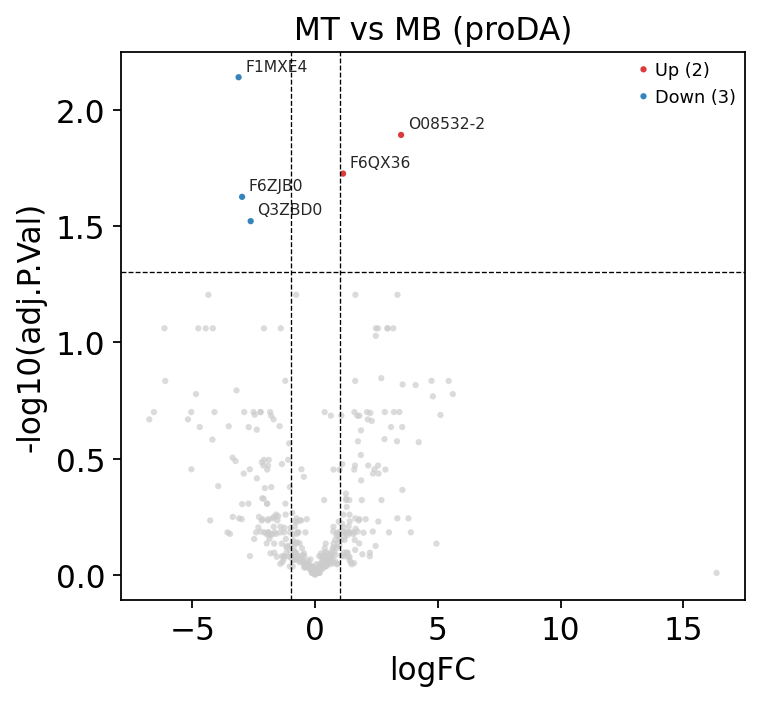
A volcano plot shows effect size (logFC) against significance for every protein at once — the standard first look. A heatmap of the top differential proteins then confirms the hits are coherent: replicates within a group should agree and the two groups should look different.

ov.protein.volcano(res, fc_col='logFC', p_col='adj.P.Val',
                   logfc_threshold=1.0, adj_p_threshold=0.05,
                   title='MT vs MB (proDA)')
plt.show()

ov.protein.heatmap(adata, de_table=res, group='group', n_top=40)
plt.show()

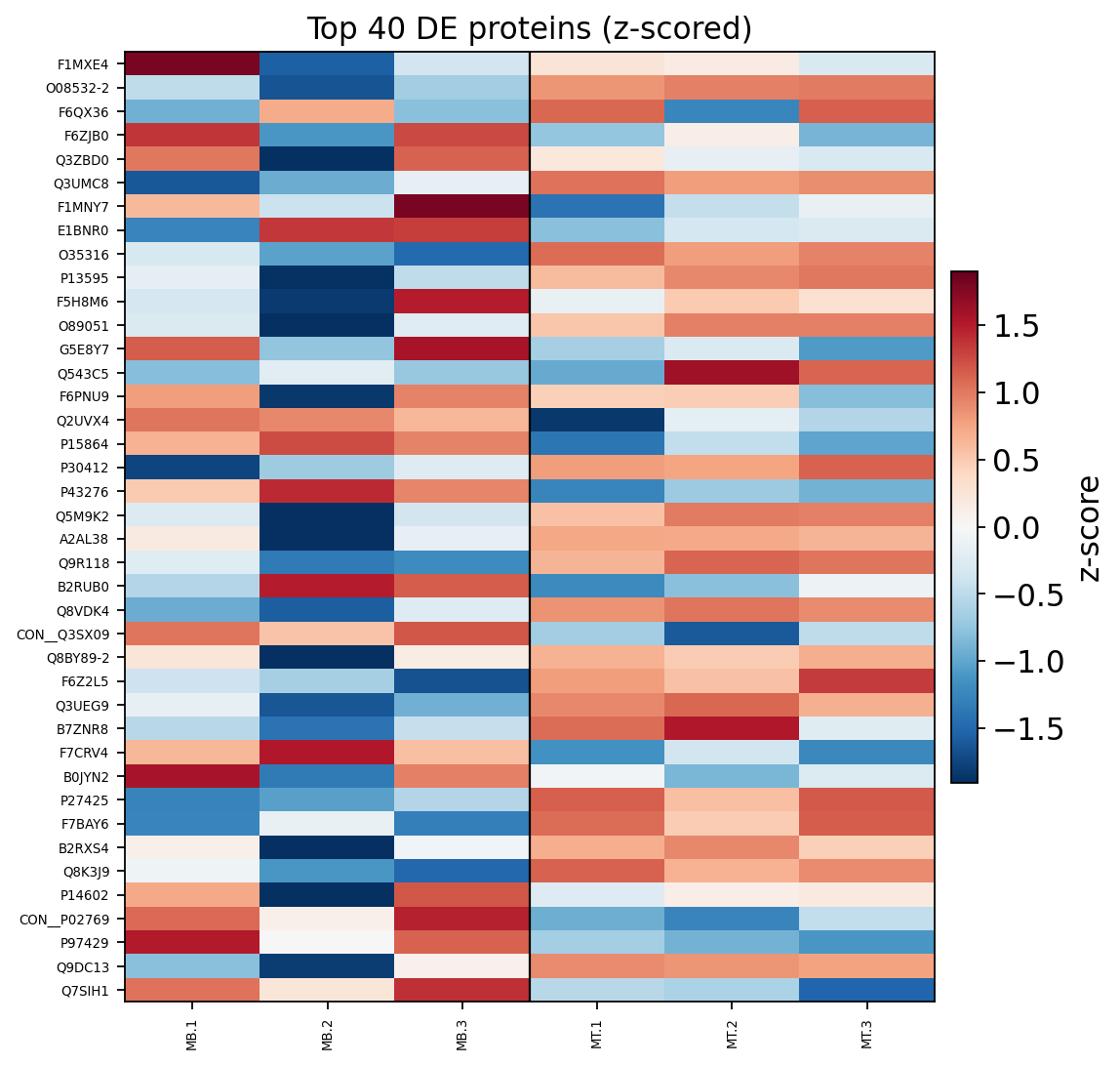
In the heatmap the three MB replicates cluster apart from the three MT replicates, and the top-40 proteins split into clean up- and down-regulated blocks. That block structure is the visual confirmation that the differential signal is real and reproducible across replicates — not driven by one outlier sample.

8. Functional enrichment

A DE list is a list of proteins; biology lives in pathways. ov.protein.enrich forwards the DE table to the ov.es enrichment engine, with method= selecting the algorithm:

• ora — over-representation analysis (Fisher-style): is a gene set enriched among the significant proteins?

• gsea — gene-set enrichment on the ranked list (no significance cutoff needed).

• ulm — univariate linear model scoring.

In a real study you would pass curated databases — MSigDB Hallmark, GO Biological Process, or KEGG — as the signatures dictionary (ov.utils.geneset_prepare loads GMT files). Here, to keep the tutorial self-contained, we build two illustrative sets straight from this dataset’s protein IDs: the top-30 up-regulated proteins (which must come out enriched — a positive control) and a random set of 30 (which should not — a negative control). Seeing the positive control light up and the random set stay flat confirms the enrichment call is wired up correctly.

up30 = res[res['logFC'] > 0].sort_values('P.Value')['gene'].head(30).tolist()
rng = np.random.default_rng(0)
rand30 = rng.choice(res['gene'].to_numpy(), size=30, replace=False).tolist()
signatures = {'Top30_up_regulated': up30, 'Random_control_set': rand30}
print('signature sizes:', {k: len(v) for k, v in signatures.items()})

signature sizes: {'Top30_up_regulated': 30, 'Random_control_set': 30}

enr = ov.protein.enrich(res, signatures=signatures, method='ora')
scores, pvals = enr
enr_table = pd.DataFrame({'enrichment_score': scores.iloc[0],
                          'p_value': pvals.iloc[0]})
enr_table.sort_values('p_value')

	enrichment_score	p_value
Top30_up_regulated	8.135843	0.000000e+00
Random_control_set	5.953753	6.570192e-39

As designed, the top-30 up-regulated set is strongly enriched among the significant proteins while the random set is not — the controls behave, so the enrichment plumbing is correct. Swap signatures for MSigDB / GO / KEGG and this same call returns interpretable biology. For a ranked-list analysis without a cutoff, switch to method='gsea'.

Summary — the best-practice recipe

The complete, defensible bulk-proteomics pipeline in ov.protein:

import omicverse as ov

# 1. load (or use read_maxquant / read_diann / read_fragpipe)
adata = ov.datasets.protein_pxd000022()

# 2. QC — drop sparsely-observed proteins
ov.protein.qc_filter(adata, min_peptides=2, min_valid=0.5)

# 3. DIAGNOSE missingness BEFORE touching it
ov.protein.missing_pattern(adata)
mcar_mask, threshold = ov.protein.model_selector(adata)

# 4. normalize away per-run loading + log2
ov.protein.normalize(adata, method='median', log2=True)

# 5. impute with a method that MATCHES the mechanism (MNAR -> qrilc)
ov.protein.impute(adata, method='qrilc', seed=0)

# 6. differential expression — proDA models dropout directly
res = ov.protein.de(adata, group='group', method='proda', reference='MB')

# 7. + 8. visualize and interpret
ov.protein.volcano(res); ov.protein.heatmap(adata, de_table=res, group='group')
ov.protein.enrich(res, signatures=msigdb_hallmark, method='ora')

The four decisions that make or break the analysis

1. Diagnose missingness before imputing. The missing-value mechanism is the most consequential property of a proteomics dataset. Look at the abundance–missingness correlation; do not assume.

2. Match the imputer to the mechanism. MNAR / left-censored → qrilc / mindet / minprob. MCAR → knn / svd. Using a KNN imputer on MNAR data invents mid-range values for undetected proteins and fabricates differential expression.

3. Normalize away per-run loading. Median (or quantile) alignment plus a log2 transform must precede every sample-to-sample comparison — otherwise loading masquerades as biology.

4. Pick the DE method for your data. Genuinely MNAR + small n → proda (models dropout, needs no imputation). Peptide-count matrix → deqms. Plain welch_t is a baseline, not a recommendation.

Continue with the other ov.protein tutorials

• t_protein_02_missing_values — missing-value theory in depth: benchmarking all nine imputers by artificial masking, and how the imputer changes the DE result.

• t_protein_03_summarization_dia — going from peptide/feature-level search output to a protein matrix; DDA and DIA.

• t_protein_04_differential_expression — DEqMS vs proDA vs MSstats vs limma vs t-test, the peptide-count–variance relationship, multi-group contrasts, and power analysis.

• t_protein_05_olink — the Olink NPX affinity-proteomics workflow (QC, LOD, bridge normalization, LMM).