Metabolite cell-cell communication in a tumour microenvironment

The companion tutorial scored metabolism within each cell. Here we ask the question that needs the whole ecosystem: in a head & neck tumour, which cell types feed which — which metabolites flow from which sender to which receiver? ov.single.MetaboliteCCC wraps MEBOCOST to infer metabolite-mediated cell-cell communication, and reuses the ov.pl.ccc_* communication plots.

Part.1 The idea behind MEBOCOST

A metabolite-mediated communication event has two ends:

• a sender cell type that makes a metabolite available — read out as high expression of its synthesising / exporting enzymes;

• a receiver cell type that takes it up or senses it — high expression of a matching sensor: a transporter, a cell-surface receptor or a nuclear receptor.

MEBOCOST estimates per-cell-type metabolite abundance from enzyme expression, pairs metabolites with sensors through a curated database, and scores every sender to receiver event against a permutation null. Tumour metabolism is not cell-autonomous — malignant cells, fibroblasts and immune cells feed and starve one another, and this is how that traffic is mapped.

import omicverse as ov

ov.plot_set()

🔬 Starting plot initialization...
🧬 Detecting GPU devices…
🚫 No GPU devices found (CUDA/MPS/ROCm/XPU)

   ____            _     _    __                  
  / __ \____ ___  (_)___| |  / /__  _____________ 
 / / / / __ `__ \/ / ___/ | / / _ \/ ___/ ___/ _ \ 
/ /_/ / / / / / / / /__ | |/ /  __/ /  (__  )  __/ 
\____/_/ /_/ /_/_/\___/ |___/\___/_/  /____/\___/                                              

🔖 Version: 2.2.1rc1   📚 Tutorials: https://omicverse.readthedocs.io/
✅ plot_set complete.

Part.2 The HNSC tumour atlas

The same Puram et al. 2017 head & neck cancer atlas (GSE103322) used by the per-cell metabolism tutorial — 5,578 cells, malignant plus the stromal and immune microenvironment.

adata = ov.datasets.metabolism_hnsc()
adata.obs['celltype'].value_counts()

🔍 Downloading data to ./data/hnsc_puram2017_full.h5ad
⚠️ File ./data/hnsc_puram2017_full.h5ad already exists

celltype
Malignant      2215
Fibroblast     1440
T cell         1237
Endothelial     260
B cell          138
Mast            120
Macrophage       98
Dendritic        51
myocyte          19
Name: count, dtype: int64

Part.3 Infer metabolite communication

ov.single.MetaboliteCCC takes the cell-type column as the unit of communication. run() estimates metabolite abundance, pairs metabolites with sensors and runs the permutation test. min_cell_number drops cell types too small to estimate from, and n_shuffle sizes the null (1000 for a publication; 100 here to keep the tutorial quick).

mccc = ov.single.MetaboliteCCC(adata, group_key='celltype')
mccc.run(n_shuffle=100, min_cell_number=30, verbose=False)

<omicverse.single._metabolism.MetaboliteCCC at 0x7f594e709780>

# the strongest metabolite -> sensor communication events
mccc.result.nlargest(10, 'Commu_Score')[
    ['Sender', 'Receiver', 'Metabolite_Name', 'Sensor',
     'Commu_Score', 'permutation_test_fdr']]

	Sender	Receiver	Metabolite_Name	Sensor	Commu_Score	permutation_test_fdr
73	Mast	Malignant	L-Glutamine	SLC3A2	20.723214	0.0
37	Macrophage	Malignant	L-Glutamine	SLC3A2	19.115429	0.0
76	Mast	Macrophage	L-Glutamine	SLC3A2	14.312806	0.0
74	Mast	B cell	L-Glutamine	SLC3A2	14.117096	0.0
72	Mast	Fibroblast	L-Glutamine	SLC38A2	13.493294	0.0
40	Macrophage	Macrophage	L-Glutamine	SLC3A2	13.202364	0.0
74	Mast	B cell	L-Glutamine	SLC38A2	13.141793	0.0
38	Macrophage	B cell	L-Glutamine	SLC3A2	13.021839	0.0
10	Malignant	Malignant	L-Glutamine	SLC3A2	12.874932	0.0
52	Endothelial	Dendritic	Farnesyl pyrophosphate	GPR183	12.629885	0.0

Part.4 The communication network

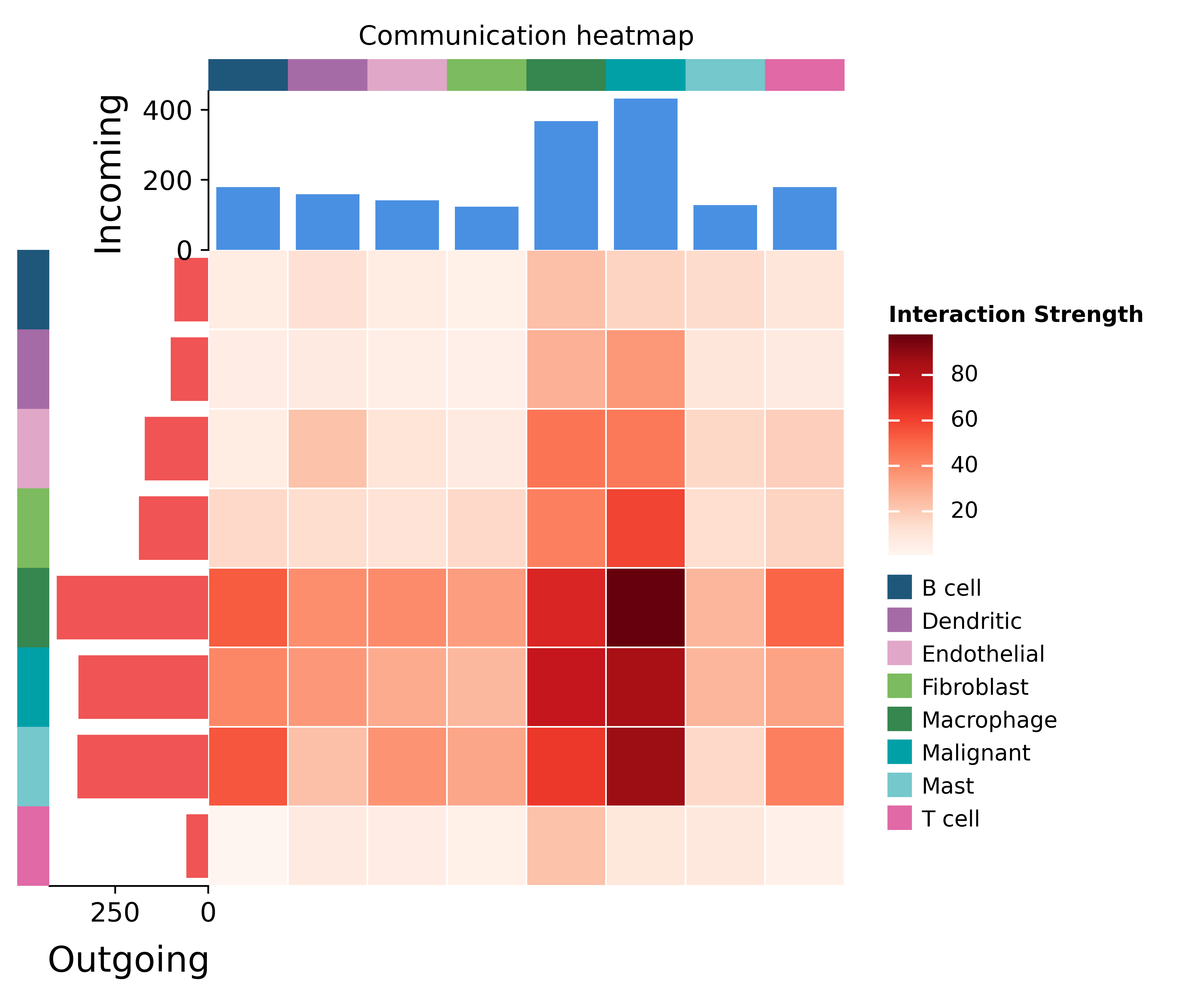
to_comm_adata() converts the MEBOCOST result into a communication AnnData — the schema the ov.pl.ccc_* plots consume. The heatmap sums communication strength over every sender to receiver pair; a bright row is a metabolite source, a bright column a sink.

comm = mccc.to_comm_adata()
fig, ax = ov.pl.ccc_heatmap(comm, plot_type='heatmap')
fig

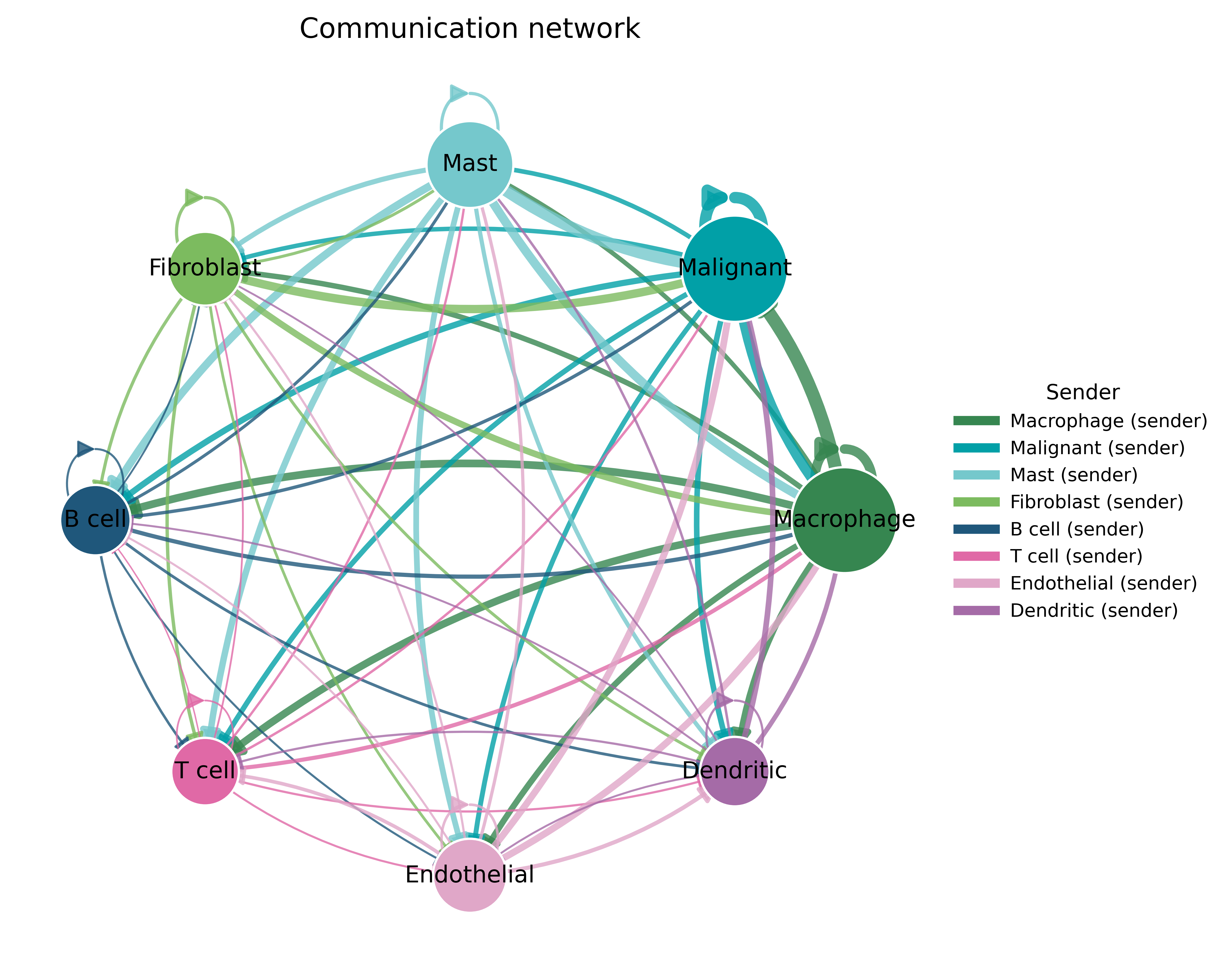
The same traffic as a directed network — arrows run from metabolite senders to receivers, weighted by communication strength.

fig, ax = ov.pl.ccc_network_plot(comm, plot_type='circle')
fig

Part.5 Drill into specific metabolite-sensor channels

The aggregated views in Part.4 confirm that signal is flowing — they do not say what is in the bottle. Every row of mccc.result names a specific (metabolite, sensor) pair, and to_comm_adata() keeps that resolution: metabolites land in the gene_a / ligand slot of the comm AnnData, sensors in gene_b / receptor. That makes the entire interaction-level ov.pl.ccc_* family — the same plots used by the LIANA ligand-receptor tutorial — available on a metabolite-CCC result.

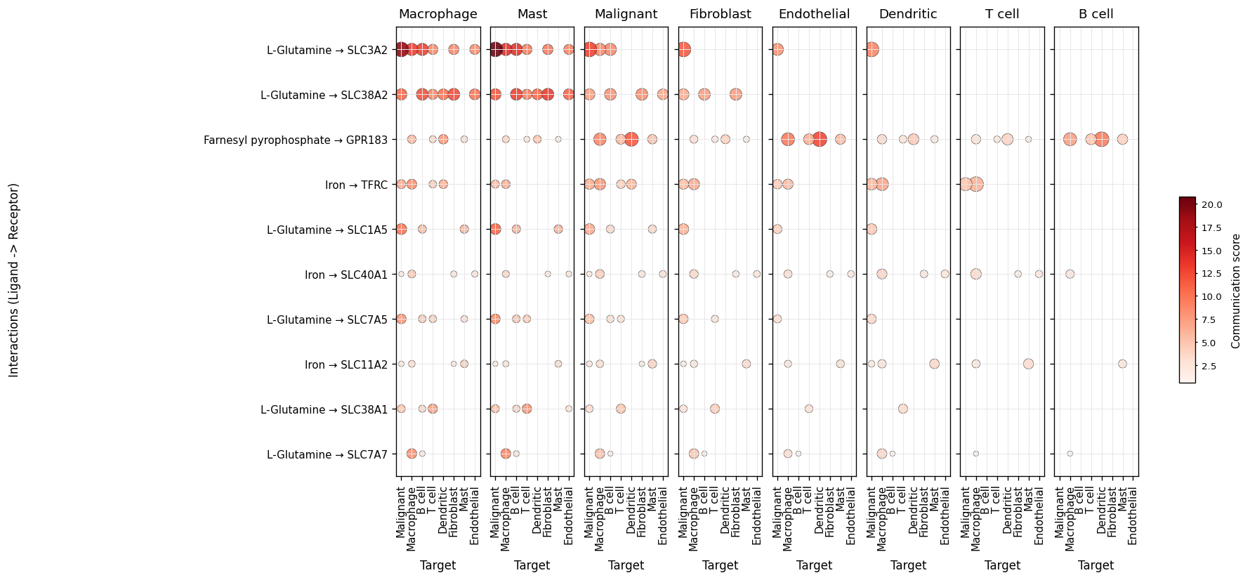
The default interaction-level view is the LIANA-style dot plot. Rows are metabolite → sensor pairs, columns are receivers, facets are senders. Dot size encodes −log10(FDR), color encodes the score.

fig, ax = ov.pl.ccc_heatmap(
    comm, plot_type='dot', display_by='interaction',
    top_n=10, pvalue_threshold=0.05,
    figsize=(16, 6.5), show=False)
fig

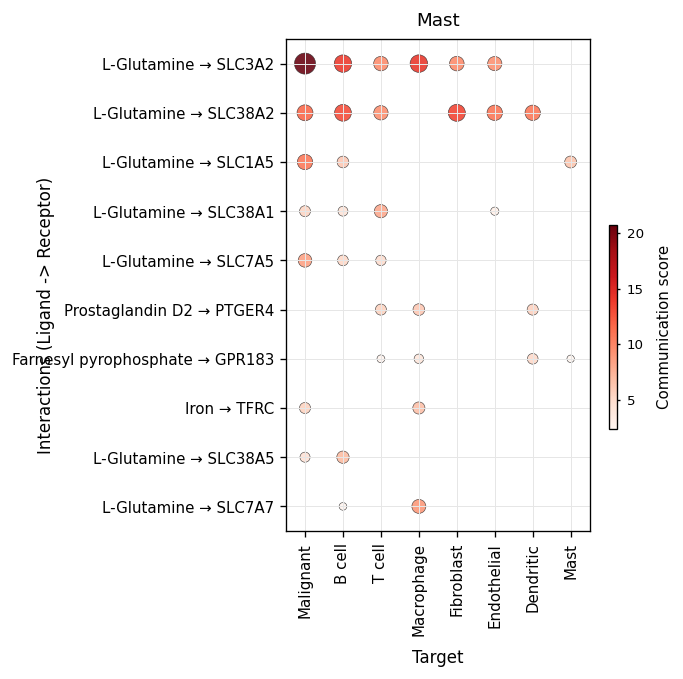
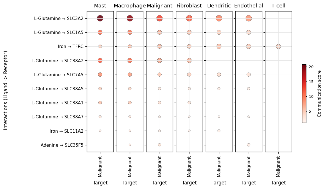
Sender / receiver focus

Once a cell type of interest is in mind, restrict the same plot to that role. sender_use=['Mast'] asks “of everything Mast cells put into the system, what dominates?”. receiver_use=['Malignant'] asks the symmetric question — who and what is feeding the tumour.

fig, ax = ov.pl.ccc_heatmap(
    comm, plot_type='dot', display_by='interaction',
    sender_use=['Mast'], top_n=10, pvalue_threshold=0.05,
    figsize=(5.5, 5), show=False)
fig

fig, ax = ov.pl.ccc_heatmap(
    comm, plot_type='dot', display_by='interaction',
    receiver_use=['Malignant'], top_n=10, pvalue_threshold=0.05,
    figsize=(10, 5), show=False)
fig

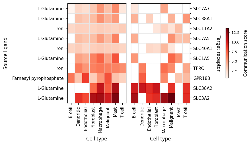
Part.6 Production vs sensing — tile + bar

tile puts the two ends of the channel side by side: left is what the sender produces (metabolite abundance), right is what the receiver expresses (sensor expression). A channel is a real signal only when both panels light up for the same (metabolite → sensor) row.

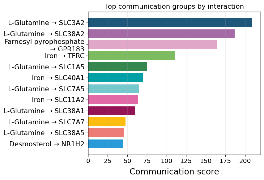
bar then collapses the matrix to a flat ranking — the strongest individual interactions across the system, useful for picking the next channel to drill into.

fig, ax = ov.pl.ccc_heatmap(
    comm, plot_type='tile', display_by='interaction',
    top_n=10, pvalue_threshold=0.05,
    figsize=(7, 4), show=False)
fig

fig, ax = ov.pl.ccc_stat_plot(
    comm, plot_type='bar', display_by='interaction',
    group_by='interaction', top_n=12,
    figsize=(6, 5), show=False)
fig

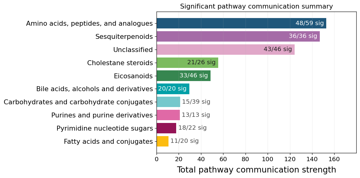
Part.7 Metabolite classes shape the landscape

HMDB’s chemical classification is joined onto the comm AnnData as var['classification'] (sub_class — e.g. “Amino acids, peptides, and analogues”, “Carbohydrates and carbohydrate conjugates”) and var['classification_super'] (super_class). Aggregating by class turns the long list of individual channels into a small set of metabolic programs: which broad class of metabolites is most active across the system.

pathway_summary ranks classes by total communication strength and annotates each bar with n_significant / n_active cell-pairs — a single-glance way to see which class of metabolites carries the most traffic and how widely it reaches.

fig, ax = ov.pl.ccc_stat_plot(
    comm, plot_type='pathway_summary',
    top_n=10, figsize=(7, 5), show=False)
fig

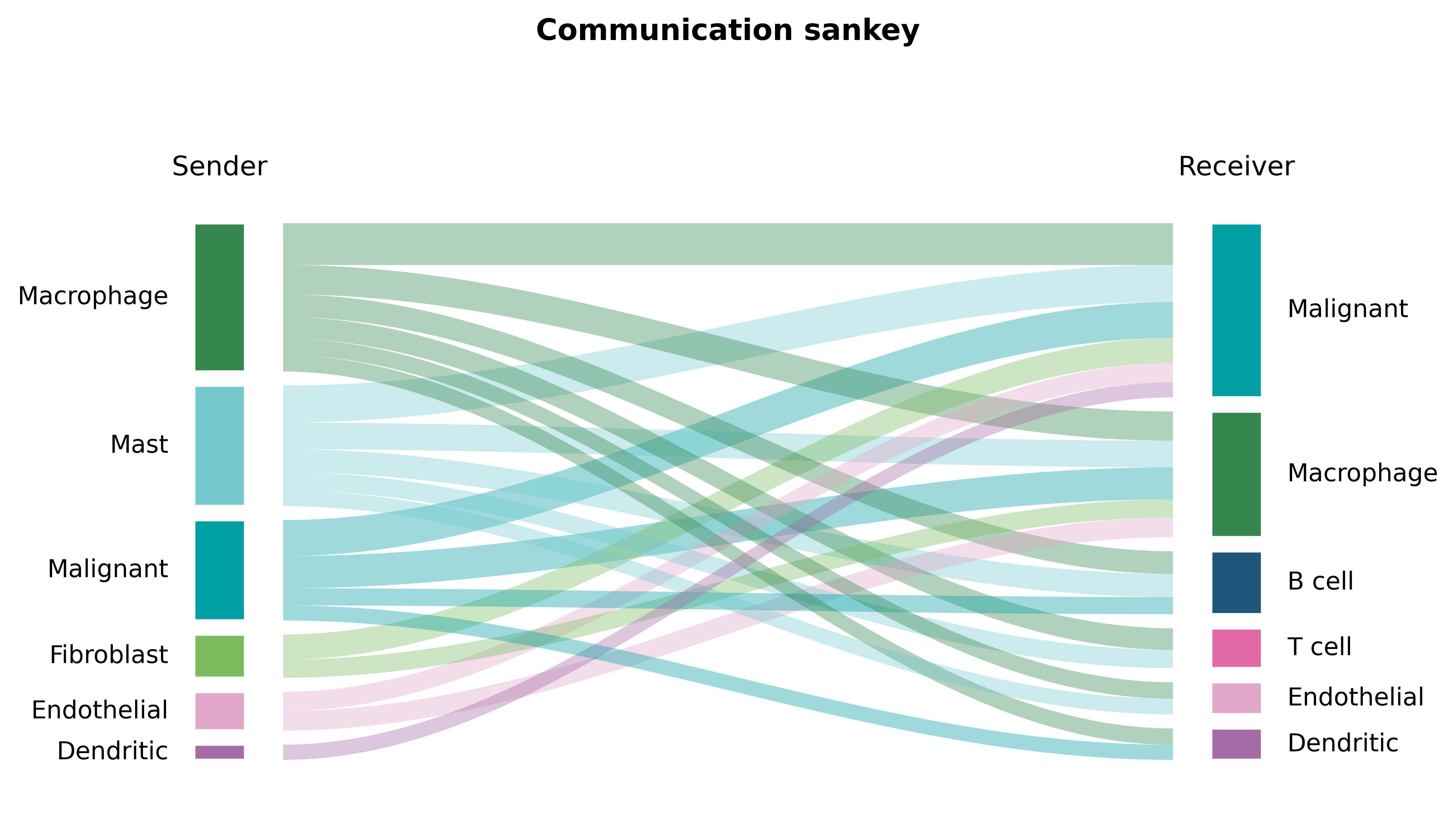
Part.8 The dominant metabolite channels

A Sankey view follows the flow end-to-end: which cell types pour the most metabolite signal into which receivers.

fig, ax = ov.pl.ccc_stat_plot(comm, plot_type='sankey')
fig

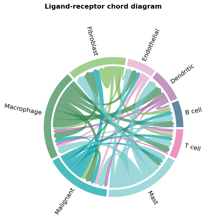
Part.9 A closer look — L-Glutamine

Reading the top events again: they nearly all converge on one channel — malignant cells receiving L-glutamine. The sensors are SLC3A2 (CD98hc), SLC1A5 and SLC38A2 — amino-acid transporters, not receptors — so MEBOCOST is reading metabolite uptake. This is textbook cancer biology: tumour cells are “glutamine-addicted”, and the analysis names who pays for the habit.

Filter the comm AnnData to the L-Glutamine channels and draw a sender-receiver chord — every L-Glutamine → sensor pair in one view.

gln_interactions = [v for v in comm.var_names if v.startswith('L-Glutamine')]
fig, ax = ov.pl.ccc_network_plot(
    comm, plot_type='lr_chord',
    pair_lr_use=gln_interactions,
    figsize=(6, 6), show=False)
fig

recv = mccc.result[mccc.result['Receiver'] == 'Malignant']
(recv.groupby('Metabolite_Name')['Commu_Score'].sum()
     .sort_values(ascending=False).head(10))

Metabolite_Name
L-Glutamine                246.935687
Iron                        53.167821
Leukotriene B4              12.561020
gamma-Aminobutyric acid      9.449661
L-Serine                     8.482404
3-Hydroxybutyric acid        7.552795
Adenine                      7.424385
D-Mannose                    7.241953
Desmosterol                  6.615091
Cholesterol                  6.119173
Name: Commu_Score, dtype: float64

import matplotlib.pyplot as plt
plt.close('all')   # clear figures left open by the ccc_* plots
gln = mccc.result.query("Receiver == 'Malignant' "
                        "and Metabolite_Name == 'L-Glutamine'")
supply = gln.groupby('Sender')['Commu_Score'].sum().sort_values()
supply.plot.barh(color='#55A868', figsize=(5, 3),
                 xlabel='glutamine communication score',
                 title='Who feeds glutamine to the tumour')
plt.show()

---

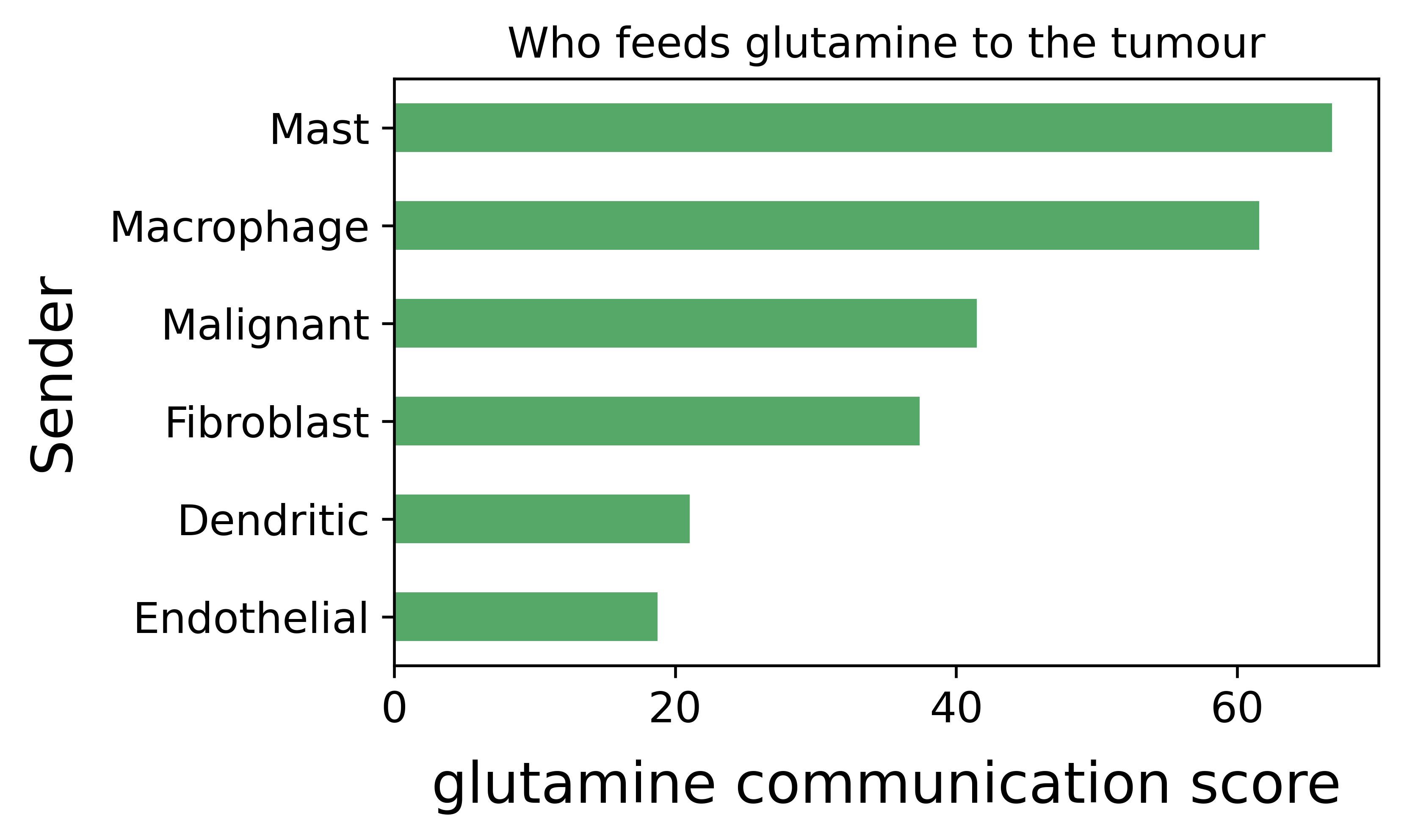
Recap

ov.single.MetaboliteCCC lifts the metabolism analysis from the single cell to the metabolic ecology of the tumour. On this head & neck cancer atlas it recovers a real dependency: the malignant compartment is a metabolite sink, and mast cells and macrophages are the chief suppliers of the L-glutamine that glutamine-addicted tumour cells consume.

The comm AnnData built by MetaboliteCCC.to_comm_adata() keeps every (metabolite, sensor) pair as its own column — metabolites in the ligand slot, sensors in the receptor slot, HMDB sub/super-class in the classification slot. That schema is what unlocks the full interaction-level ov.pl.ccc_* family in this tutorial: the dot / tile / bar / pathway-bubble / chord views are the same plots the LIANA tutorial uses on protein ligand-receptor pairs, applied here to metabolite channels.

Paired with the per-cell scMetabolism / scFEA analysis, it completes the picture — metabolic state within cells and metabolite exchange between them.