Peak-to-gene linkage (multiome)

Peak-to-gene linkage (multiome)#

A scATAC peak is only useful once you know which gene it regulates. With paired RNA + ATAC (10x multiome) we can learn those links directly: for each peak–gene pair within a genomic window, correlate peak accessibility against gene expression across metacells, and keep the significant correlations. This is the ArchR / addPeak2GeneLinks idea, exposed in ov.epi as ov.epi.tl.peak_to_gene.

This tutorial uses the public 10x PBMC 10k multiome dataset (paired scRNA + scATAC, GRCh38), which ov.epi.datasets downloads on demand:

load the paired ATAC peak matrix + RNA matrix
build an ATAC embedding with iterative LSI
correlate peaks with genes (ov.epi.tl.peak_to_gene)
visualise the links around marker genes with ov.epi.pl.plot_peak2gene

import warnings
warnings.filterwarnings('ignore')

import numpy as np
import pandas as pd
import matplotlib.pyplot as plt

import omicverse as ov
ov.epi.pl.plot_set()
print('omicverse', ov.__version__)

└─ 🔬 Starting plot initialization...
  ├─ Apply Scanpy/matplotlib settings
  ├─ Custom font setup
  ├─ Suppress warnings
  ├─ 
___________      .__                      
\_   _____/_____ |__| ____   ____   ____  
 |    __)_\____ \|  |/  _ \ /    \_/ __ \ 
 |        \  |_> >  (  <_> )   |  \  ___/ 
/_______  /   __/|__|\____/|___|  /\___  >
        \/|__|                  \/     \/ 

  ├─ 🔖 Version: 0.0.1rc1   📚 Tutorials: https://epione.readthedocs.io/
└─ ✅ plot_set complete.

omicverse 2.2.1rc1

1 · Load the paired multiome data#

ov.epi.datasets.pbmc10k_multiome() returns two AnnData objects sharing the same cell barcodes — an ATAC peak matrix and an RNA count matrix, both already annotated with cell_type.

atac, rna = ov.epi.datasets.pbmc10k_multiome()
print('ATAC:', atac.shape, '| RNA:', rna.shape)
print('paired barcodes:', bool((atac.obs_names == rna.obs_names).all()))
atac.obs['cell_type'].value_counts().head()

ATAC: (9631, 107194) | RNA: (9631, 29095)
paired barcodes: True

cell_type
CD14 Mono    2554
CD4 Naive    1382
CD8 Naive    1354
CD4 TCM      1113
CD16 Mono     442
Name: count, dtype: int64

2 · Gene and exon annotation#

Both peak_to_gene (to find each gene’s TSS) and the linkage plot (to draw the gene model) need a gene/exon annotation table. We read it from the bundled GRCh38 Gencode GFF3 with pyranges.

import pyranges as pr

gtf_path = ov.epi.data.hg38.annotation
g = pr.read_gff3(str(gtf_path)).df

def _ann(feature):
    sub = g[g.Feature == feature]
    return pd.DataFrame({
        'gene_name': sub['gene_name'].astype(str).values,
        'chrom':     sub['Chromosome'].astype(str).values,
        'start':     sub['Start'].astype(int).values,
        'end':       sub['End'].astype(int).values,
        'strand':    sub['Strand'].astype(str).values,
    })

gene_ann = _ann('gene')
exon_ann = _ann('exon')
print('genes:', len(gene_ann), '| exons:', len(exon_ann))

genes: 61852 | exons: 839796

3 · ATAC embedding#

peak_to_gene groups cells into metacells using a low-dimensional embedding; we compute the standard ArchR-style iterative LSI on the ATAC peaks.

ov.epi.tl.iterative_lsi(atac, n_components=30, iterations=2, var_features=25000,
                        resolution=0.5, n_neighbors=30, seed=1)
print('ATAC embedding:', atac.obsm['X_iterative_lsi'].shape)

└─ [iterative_lsi] Initial feature set: 106,658 / 107,194
└─ [iterative_lsi] Iter 1/2 | fit on 9,631 cells x 106,658 features
computing neighbors
finished: added to `.uns['neighbors']`
    `.obsp['distances']`, distances for each pair of neighbors
    `.obsp['connectivities']`, weighted adjacency matrix (0:00:32)
running Leiden clustering
finished: found 14 clusters and added
    'leiden', the cluster labels (adata.obs, categorical) (0:00:00)
└─ [iterative_lsi]   -> 14 clusters; selected 25,000 variable features for next round
└─ [iterative_lsi] Iter 2/2 | fit on 9,631 cells x 25,000 features
└─ [iterative_lsi] Done. Stored embedding (9,631 x 29) in adata.obsm['X_iterative_lsi']
ATAC embedding: (9631, 29)

4 · Correlate peaks with genes#

ov.epi.tl.peak_to_gene aggregates cells into metacells, then correlates each peak with every gene whose TSS lies within max_distance (250 kb) of the peak, returning a tidy table of links with a correlation, p-value and FDR.

links = ov.epi.tl.peak_to_gene(
    atac, rna=rna, gene_annotation=gene_ann,
    use_rep='X_iterative_lsi',
    n_metacells=500, k_neighbors=100, max_distance=250_000, seed=1,
)
sig = links[links['fdr'] < 0.05]
print(f'{len(links):,} peak-gene pairs | {len(sig):,} significant (FDR < 0.05)')
links.head()

└─ [peak_to_gene] 107,194 peaks | 20,169 annotated genes | 9,631 cells
  └─ [peak_to_gene] Building 500 metacells × 100 neighbours from X_iterative_lsi
  └─ [peak_to_gene] Aggregating peak matrix
└─ [peak_to_gene] Aggregating gene matrix
└─ [peak_to_gene] Finding peak-gene pairs within ±250,000 bp
└─ [peak_to_gene] 726,292 candidate pairs
  └─ [peak_to_gene] Computing correlations
└─ [peak_to_gene] 726,292 pairs retained, 441,342 significant (FDR < 0.05)
726,292 peak-gene pairs | 441,342 significant (FDR < 0.05)

	peak	gene	chrom	peak_start	peak_end	gene_start	gene_end	tss	distance	correlation	t	p_value	fdr
0	chr1:816881-817647	LINC01409	chr1	816881	817647	778746	810065	778746	38518	0.367556	8.819705	1.937570e-17	1.153987e-16
1	chr1:816881-817647	FAM87B	chr1	816881	817647	817370	819837	817370	-106	0.214858	4.909412	1.240268e-06	3.701546e-06
2	chr1:816881-817647	LINC01128	chr1	816881	817647	825137	859446	825137	-7873	0.103890	2.331009	2.015113e-02	3.446575e-02
3	chr1:816881-817647	LINC00115	chr1	816881	817647	824227	827539	827539	-10275	0.546485	14.562097	2.831169e-40	3.955713e-39
4	chr1:816881-817647	FAM41C	chr1	816881	817647	868070	876903	876903	-59639	0.165115	3.735962	2.086407e-04	4.896519e-04

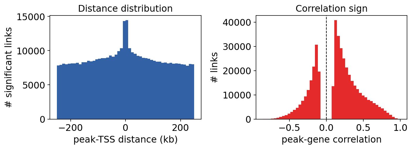
Properties of the significant links#

Two quick diagnostics: significant links are enriched at short peak–TSS distances, and positive correlations dominate (accessible enhancers tend to raise expression).

fig, axes = plt.subplots(1, 2, figsize=(9, 3.4))
axes[0].hist(sig['distance'] / 1000, bins=50, color='#3361A5')
axes[0].set_xlabel('peak-TSS distance (kb)'); axes[0].set_ylabel('# significant links')
axes[0].set_title('Distance distribution')

axes[1].hist(sig['correlation'], bins=50, color='#E42A2A')
axes[1].axvline(0, color='k', lw=1, ls='--')
axes[1].set_xlabel('peak-gene correlation'); axes[1].set_ylabel('# links')
axes[1].set_title('Correlation sign')
plt.tight_layout(); plt.show()

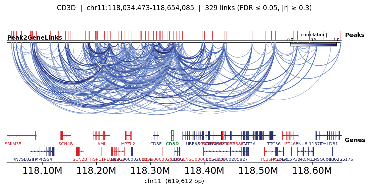
../_images/9e390bc489aa41d42effe7102c9096227dbc72f7d4cf2af61a41493c01188681.png

5 · Visualise links around marker genes#

ov.epi.pl.plot_peak2gene draws a genome-browser-style panel: the gene model, the peaks, and arcs connecting each peak to the gene coloured by correlation. CD3D is a pan-T-cell gene.

fig, _ = ov.epi.pl.plot_peak2gene(
    atac, gene='CD3D',
    gene_annotation=gene_ann, exon_annotation=exon_ann,
    fdr_thresh=0.05, min_abs_r=0.3, pad_bp=80_000, figsize=(8, 4), show=False,
)
plt.tight_layout(); plt.show()

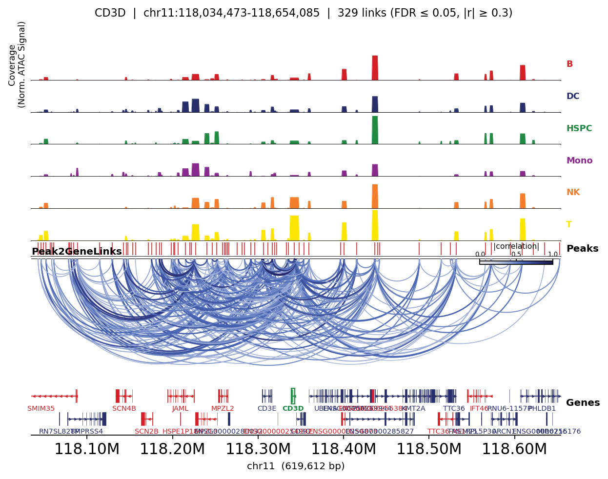
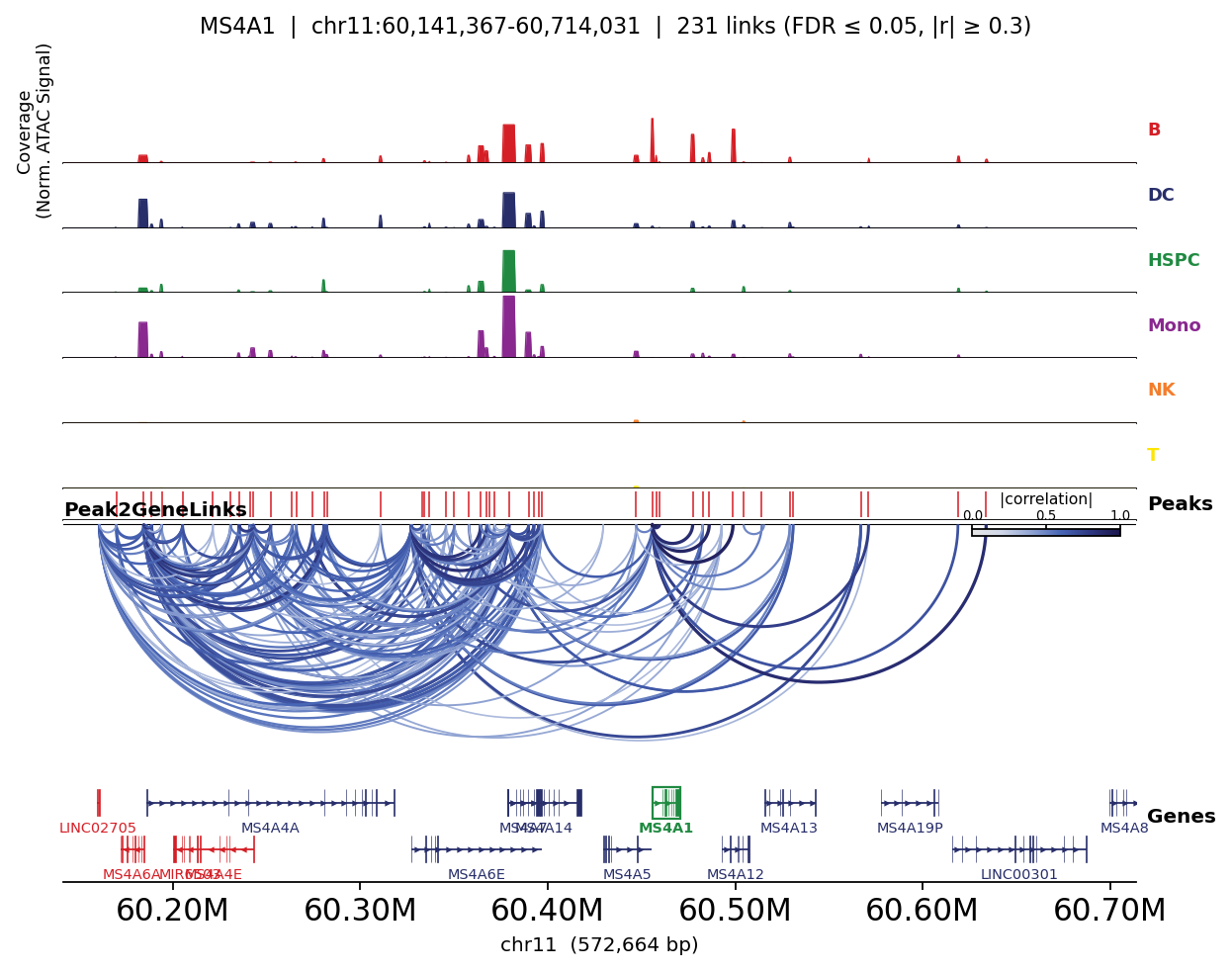
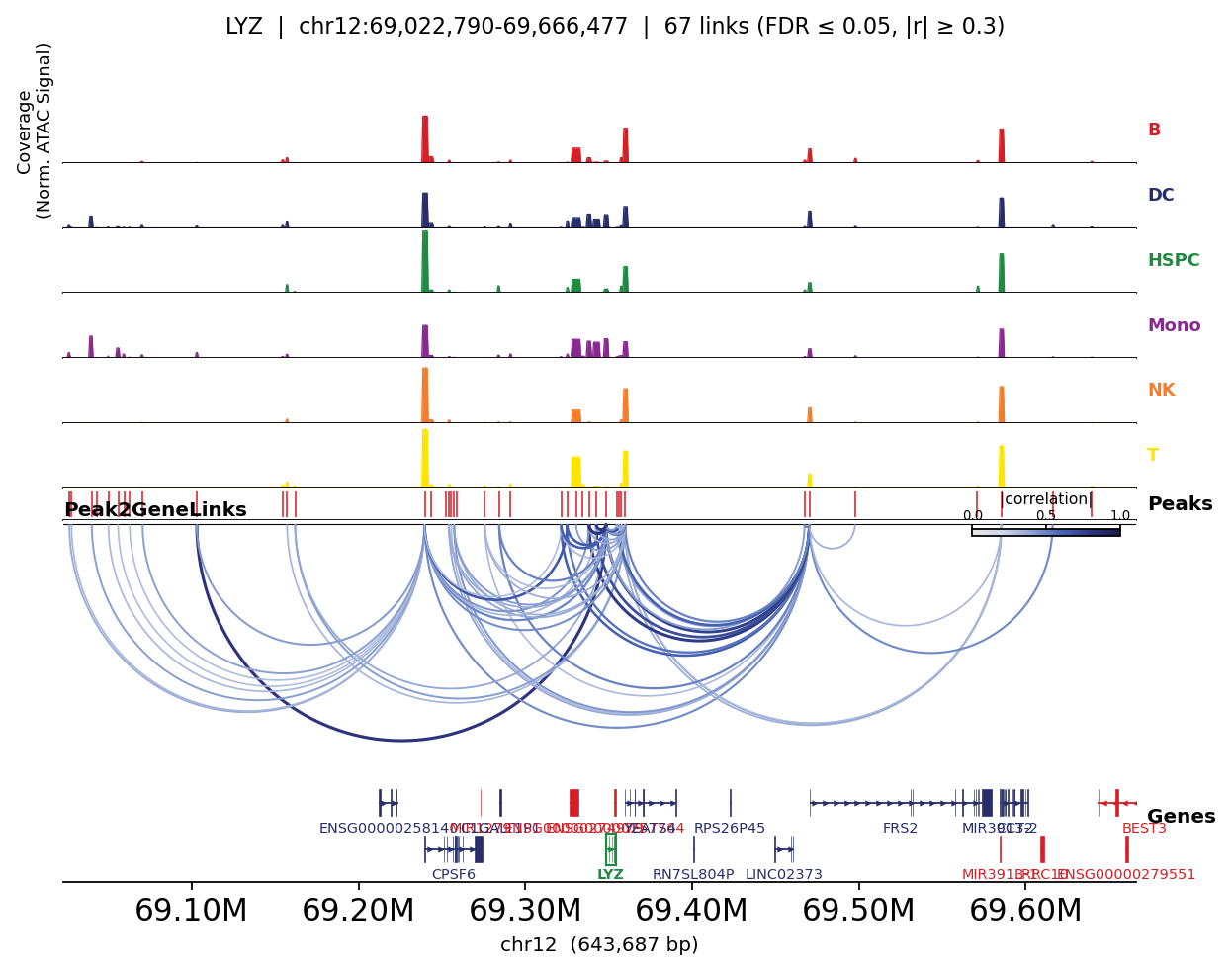
../_images/239b4cd675dfe9370a71a654a2b5189a2efe5c5cce95076aa5110ed715386faf.png

Links coloured by lineage accessibility#

Mapping the fine-grained cell_type to broad lineages lets the plot also show per-lineage peak accessibility — so you can see, for each marker, that its linked peaks open specifically in the matching lineage.

major = {
    'CD4 Naive':'T','CD4 TCM':'T','CD4 TEM':'T','Treg':'T','CD8 Naive':'T',
    'CD8 TEM_1':'T','CD8 TEM_2':'T','MAIT':'T','gdT':'T',
    'Naive B':'B','Memory B':'B','Intermediate B':'B','Plasma':'B',
    'NK':'NK','CD14 Mono':'Mono','CD16 Mono':'Mono','cDC':'DC','pDC':'DC','HSPC':'HSPC',
}
atac.obs['lineage'] = atac.obs['cell_type'].map(major).fillna('other').astype('category')

for gene in ['CD3D', 'MS4A1', 'LYZ']:
    fig, _ = ov.epi.pl.plot_peak2gene(
        atac, gene=gene, group_by='lineage',
        gene_annotation=gene_ann, exon_annotation=exon_ann,
        fdr_thresh=0.05, min_abs_r=0.3, pad_bp=80_000, figsize=(8, 4), show=False,
    )
    plt.tight_layout(); plt.show()

../_images/7e9e5841e608a522a72747f1cb1dede5d3b73aa832e84abb5339435050088bc1.png

../_images/d43252af9200724ea208259fb01c682bd63f9341a541a1768fc647d10ac9a948.png

../_images/8569f2d8084e472ce4125a0241015b06227ae9dbc63ca1230496d286e2e64055.png

Summary#

stage	function
load paired RNA+ATAC	`ov.epi.datasets.pbmc10k_multiome`
ATAC embedding	`ov.epi.tl.iterative_lsi`
peak↔gene correlation	`ov.epi.tl.peak_to_gene`
linkage plot	`ov.epi.pl.plot_peak2gene`

Peak-to-gene links turn an anonymous accessibility peak into a candidate regulatory element for a named gene — the foundation for enhancer-driven gene-regulatory analysis.