Side-by-side comparison of all metacell backends#
Each backend in the metacell-zoo was developed by a different
group with different assumptions. This notebook runs all six
always-available backends (seacells, metaq, supercell, kmeans,
random, geosketch) on the same pancreas data and ranks them by:
runtime — how long does it take?
purity — fraction of each metacell that belongs to a single celltype
rigor_score — mcRigor’s composite score (higher = better)
dubious_rate — fraction of cells in heterogeneous metacells
compactness — mean distance from cells to their metacell centroid in PCA space
ov.single.compare_metacell_backends runs all of this in one call.
1. Setup#
# Standard imports + omicverse defaults.
import warnings
warnings.filterwarnings('ignore')

import numpy as np
import pandas as pd
import omicverse as ov
import scvelo as scv      # only used for the demo dataset

ov.plot_set()
🔬 Starting plot initialization...
🧬 Detecting GPU devices…
✅ NVIDIA CUDA GPUs detected: 1
    • [CUDA 0] NVIDIA H100 80GB HBM3
      Memory: 79.1 GB | Compute: 9.0

   ____            _     _    __
  / __ \____ ___  (_)___| |  / /__  _____________
 / / / / __ `__ \/ / ___/ | / / _ \/ ___/ ___/ _ \
/ /_/ / / / / / / / /__ | |/ /  __/ /  (__  )  __/
\____/_/ /_/ /_/_/\___/ |___/\___/_/  /____/\___/

🔖 Version: 2.2.0   📚 Tutorials: https://omicverse.readthedocs.io/
✅ plot_set complete.
2. Load and preprocess#
# Pancreas scRNA-seq (Bastidas-Ponce et al. 2019). Standard omicverse
# preprocess flow: qc -> preprocess -> scale -> pca -> neighbors -> umap.
adata = scv.datasets.pancreas()
adata = ov.pp.qc(adata,
                 tresh={'mito_perc': 0.20, 'nUMIs': 500, 'detected_genes': 250},
                 mt_startswith='mt-')
adata = ov.pp.preprocess(adata, mode='shiftlog|pearson', n_HVGs=2000)
adata.layers['lognorm'] = adata.X.copy()        # mcRigor reads this
adata = adata[:, adata.var.highly_variable_features]
ov.pp.scale(adata)
ov.pp.pca(adata, layer='scaled', n_pcs=30)
adata.obsm['X_pca'] = adata.obsm['scaled|original|X_pca']
ov.pp.neighbors(adata, n_neighbors=15, use_rep='X_pca')
ov.pp.umap(adata)
print('adata:', adata.shape, 'celltypes:', sorted(adata.obs['clusters'].unique()))
🖥️ Using CPU mode for QC...

📊 Step 1: Calculating QC Metrics

   ✓ Gene Family Detection:
   ┌──────────────────────────────┬────────────────────┬────────────────────┐
   │ Gene Family                  │ Genes Found        │ Detection Method   │
   ├──────────────────────────────┼────────────────────┼────────────────────┤
   │ Mitochondrial                │ 13                 │ Auto (MT-)         │
   ├──────────────────────────────┼────────────────────┼────────────────────┤
   │ Ribosomal                    │ 0 ⚠️               │ Auto (RPS/RPL)     │
   ├──────────────────────────────┼────────────────────┼────────────────────┤
   │ Hemoglobin                   │ 0 ⚠️               │ Auto (regex)       │
   └──────────────────────────────┴────────────────────┴────────────────────┘

   ✓ QC Metrics Summary:
   ┌─────────────────────────┬────────────────────┬─────────────────────────┐
   │ Metric                  │ Mean               │ Range (Min - Max)       │
   ├─────────────────────────┼────────────────────┼─────────────────────────┤
   │ nUMIs                   │ 6675               │ 3020 - 18524            │
   ├─────────────────────────┼────────────────────┼─────────────────────────┤
   │ Detected Genes          │ 2516               │ 1473 - 4492             │
   ├─────────────────────────┼────────────────────┼─────────────────────────┤
   │ Mitochondrial %         │ 0.7%               │ 0.2% - 4.3%             │
   ├─────────────────────────┼────────────────────┼─────────────────────────┤
   │ Ribosomal %             │ 0.0%               │ 0.0% - 0.0%             │
   ├─────────────────────────┼────────────────────┼─────────────────────────┤
   │ Hemoglobin %            │ 0.0%               │ 0.0% - 0.0%             │
   └─────────────────────────┴────────────────────┴─────────────────────────┘

   📈 Original cell count: 3,696

🔧 Step 2: Quality Filtering (SEURAT)
   Thresholds: mito≤0.2, nUMIs≥500, genes≥250
   📊 Seurat Filter Results:
     • nUMIs filter (≥500): 0 cells failed (0.0%)
     • Genes filter (≥250): 0 cells failed (0.0%)
     • Mitochondrial filter (≤0.2): 0 cells failed (0.0%)
   ✓ Filters applied successfully
   ✓ Combined QC filters: 0 cells removed (0.0%)

🎯 Step 3: Final Filtering
   Parameters: min_genes=200, min_cells=3
   Ratios: max_genes_ratio=1, max_cells_ratio=1
✓ Final filtering: 0 cells, 12,261 genes removed

🔍 Step 4: Doublet Detection
   💡 Running pyscdblfinder (Python port of R scDblFinder)
   🔍 Running scdblfinder detection...
[ScDblFinder] wrote scDblFinder_score + scDblFinder_class — threshold=0.387
   ✓ scDblFinder completed: 66 doublets removed (1.8%)

╭─ SUMMARY: qc ──────────────────────────────────────────────────────╮
│  Duration: 17.1113s                                                │
│  Shape:    3,696 x 27,998 (Unchanged)                              │
│                                                                    │
│  CHANGES DETECTED                                                  │
│  ────────────────                                                  │
│  ● OBS    │ ✚ cell_complexity (float)                              │
│           │ ✚ detected_genes (int)                                 │
│           │ ✚ hb_perc (float)                                      │
│           │ ✚ mito_perc (float)                                    │
│           │ ✚ nUMIs (float)                                        │
│           │ ✚ n_counts (float)                                     │
│           │ ✚ n_genes (int)                                        │
│           │ ✚ n_genes_by_counts (int)                              │
│           │ ✚ passing_mt (bool)                                    │
│           │ ✚ passing_nUMIs (bool)                                 │
│           │ ✚ passing_ngenes (bool)                                │
│           │ ✚ pct_counts_hb (float)                                │
│           │ ✚ pct_counts_mt (float)                                │
│           │ ✚ pct_counts_ribo (float)                              │
│           │ ✚ ribo_perc (float)                                    │
│           │ ✚ total_counts (float)                                 │
│                                                                    │
│  ● VAR    │ ✚ hb (bool)                                            │
│           │ ✚ mt (bool)                                            │
│           │ ✚ ribo (bool)                                          │
│                                                                    │
╰────────────────────────────────────────────────────────────────────╯
🔍 [2026-05-19 17:38:39] Running preprocessing in 'cpu' mode...
Begin robust gene identification
    After filtration, 15737/15737 genes are kept.
    Among 15737 genes, 15736 genes are robust.
✅ Robust gene identification completed successfully.
Begin size normalization: shiftlog and HVGs selection pearson
🔍 Count Normalization:
   Target sum: 500000.0
   Exclude highly expressed: True
   Max fraction threshold: 0.2
   ⚠️ Excluding 1 highly-expressed genes from normalization computation
   Excluded genes: ['Ghrl']
✅ Count Normalization Completed Successfully!
   ✓ Processed: 3,630 cells × 15,736 genes
   ✓ Runtime: 0.25s

🔍 Highly Variable Genes Selection (Experimental):
   Method: pearson_residuals
   Target genes: 2,000
   Theta (overdispersion): 100
✅ Experimental HVG Selection Completed Successfully!
   ✓ Selected: 2,000 highly variable genes out of 15,736 total (12.7%)
   ✓ Results added to AnnData object:
     • 'highly_variable': Boolean vector (adata.var)
     • 'highly_variable_rank': Float vector (adata.var)
     • 'highly_variable_nbatches': Int vector (adata.var)
     • 'highly_variable_intersection': Boolean vector (adata.var)
     • 'means': Float vector (adata.var)
     • 'variances': Float vector (adata.var)
     • 'residual_variances': Float vector (adata.var)
    Time to analyze data in cpu: 1.46 seconds.
✅ Preprocessing completed successfully.
    Added:
        'highly_variable_features', boolean vector (adata.var)
        'means', float vector (adata.var)
        'variances', float vector (adata.var)
        'residual_variances', float vector (adata.var)
        'counts', raw counts layer (adata.layers)
    End of size normalization: shiftlog and HVGs selection pearson

╭─ SUMMARY: preprocess ──────────────────────────────────────────────╮
│  Duration: 1.857s                                                  │
│  Shape:    3,630 x 15,737 -> 3,630 x 15,736                        │
│                                                                    │
│  CHANGES DETECTED                                                  │
│  ────────────────                                                  │
│  ● VAR    │ ✚ highly_variable (bool)                               │
│           │ ✚ highly_variable_features (bool)                      │
│           │ ✚ highly_variable_rank (float)                         │
│           │ ✚ means (float)                                        │
│           │ ✚ n_cells (int)                                        │
│           │ ✚ percent_cells (float)                                │
│           │ ✚ residual_variances (float)                           │
│           │ ✚ robust (bool)                                        │
│           │ ✚ variances (float)                                    │
│                                                                    │
│  ● UNS    │ ✚ history_log                                          │
│           │ ✚ hvg                                                  │
│           │ ✚ log1p                                                │
│                                                                    │
│  ● LAYERS │ ✚ counts (sparse matrix, 3630x15736)                   │
│                                                                    │
╰────────────────────────────────────────────────────────────────────╯
╭─ SUMMARY: scale ───────────────────────────────────────────────────╮
│  Duration: 0.6593s                                                 │
│  Shape:    3,630 x 2,000 (Unchanged)                               │
│                                                                    │
│  CHANGES DETECTED                                                  │
│  ────────────────                                                  │
│  ● LAYERS │ ✚ scaled (array, 3630x2000)                            │
│                                                                    │
╰────────────────────────────────────────────────────────────────────╯
computing PCA🔍
    with n_comps=30
   🖥️ Using sklearn PCA for CPU computation
   🖥️ sklearn PCA backend: CPU computation
   📊 PCA input data type: ArrayView, shape: (3630, 2000), dtype: float64
🔧 PCA solver used: covariance_eigh
    finished✅ (1.89s)

╭─ SUMMARY: pca ─────────────────────────────────────────────────────╮
│  Duration: 1.8986s                                                 │
│  Shape:    3,630 x 2,000 (Unchanged)                               │
│                                                                    │
│  CHANGES DETECTED                                                  │
│  ────────────────                                                  │
│  ● UNS    │ ✚ scaled|original|cum_sum_eigenvalues                  │
│           │ ✚ scaled|original|pca_var_ratios                       │
│                                                                    │
│  ● OBSM   │ ✚ scaled|original|X_pca (array, 3630x30)               │
│                                                                    │
╰────────────────────────────────────────────────────────────────────╯
🖥️ Using Scanpy CPU to calculate neighbors...

🔍 K-Nearest Neighbors Graph Construction:
   Mode: cpu
   Neighbors: 15
   Method: umap
   Metric: euclidean
   Representation: X_pca
   🔍 Computing neighbor distances...
🔍 Computing connectivity matrix...
   💡 Using UMAP-style connectivity
✓ Graph is fully connected

✅ KNN Graph Construction Completed Successfully!
   ✓ Processed: 3,630 cells with 15 neighbors each
   ✓ Results added to AnnData object:
     • 'neighbors': Neighbors metadata (adata.uns)
     • 'distances': Distance matrix (adata.obsp)
     • 'connectivities': Connectivity matrix (adata.obsp)

╭─ SUMMARY: neighbors ───────────────────────────────────────────────╮
│  Duration: 8.6527s                                                 │
│  Shape:    3,630 x 2,000 (Unchanged)                               │
│                                                                    │
│  CHANGES DETECTED                                                  │
│  ────────────────                                                  │
╰────────────────────────────────────────────────────────────────────╯
🔍 [2026-05-19 17:38:53] Running UMAP in 'cpu' mode...
🖥️ Using Scanpy CPU UMAP...

🔍 UMAP Dimensionality Reduction:
   Mode: cpu
   Method: umap
   Components: 2
   Min distance: 0.5
{'n_neighbors': 15, 'method': 'umap', 'random_state': 0, 'metric': 'euclidean', 'use_rep': 'X_pca'}
   🔍 Computing UMAP parameters...
   🔍 Computing UMAP embedding (classic method)...
✅ UMAP Dimensionality Reduction Completed Successfully!
   ✓ Embedding shape: 3,630 cells × 2 dimensions
   ✓ Results added to AnnData object:
     • 'X_umap': UMAP coordinates (adata.obsm)
     • 'umap': UMAP parameters (adata.uns)
✅ UMAP completed successfully.

╭─ SUMMARY: umap ────────────────────────────────────────────────────╮
│  Duration: 0.7885s                                                 │
│  Shape:    3,630 x 2,000 (Unchanged)                               │
│                                                                    │
│  CHANGES DETECTED                                                  │
│  ────────────────                                                  │
│  ● UNS    │ ✚ umap                                                 │
│           │ └─ params: {'a': 0.5830300199950147, 'b': 1.334166993228519}│
│                                                                    │
╰────────────────────────────────────────────────────────────────────╯
adata: (3630, 2000) celltypes: ['Alpha', 'Beta', 'Delta', 'Ductal', 'Epsilon', 'Ngn3 high EP', 'Ngn3 low EP', 'Pre-endocrine']
3. The single-call benchmark#
bench = ov.single.compare_metacell_backends(
    adata,
    backends=['seacells', 'metaq', 'supercell', 'kmeans', 'random', 'geosketch'],
    n_metacells=100,
    use_rep='X_pca',
    layer='counts',
    layer_lognorm='lognorm',
    eval_label='clusters',
    device='cpu',           # seacells GPU path needs cupy
    n_rigor_rep=20,
    random_state=0,
    train_epoch=80, warm_epochs=10, codebook_init='random',  # metaq-only kwargs
)
bench[['runtime_s', 'dubious_rate', 'rigor_score',
       'mean_purity', 'mean_compactness', 'n_metacells']].round(3)
Welcome to SEACells!
Parameter graph_construction = union being used to build KNN graph...
Building kernel on X_pca
WARNING: adata.X seems to be already log-transformed.
[Epoch 1] RNA: Loss Rec=1.6497
[Epoch 1] RNA: Loss Rec=0.8152 Loss Rec Q=0.8190 | Codebook: Loss C=0.0038
[Epoch 20] RNA: Loss Rec=0.7487 Loss Rec Q=0.7667 | Codebook: Loss C=0.0095
[Epoch 40] RNA: Loss Rec=0.7331 Loss Rec Q=0.7618 | Codebook: Loss C=0.0106
[Epoch 60] RNA: Loss Rec=0.7214 Loss Rec Q=0.7591 | Codebook: Loss C=0.0104
[Epoch 80] RNA: Loss Rec=0.7126 Loss Rec Q=0.7565 | Codebook: Loss C=0.0110
| runtime_s | dubious_rate | rigor_score | mean_purity | mean_compactness | n_metacells | |
|---|---|---|---|---|---|---|
| backend | ||||||
| seacells | 16.119 | 0.653 | 0.420 | 0.896 | 8.044 | 100 |
| metaq | 424.741 | 0.695 | 0.400 | 0.879 | 8.791 | 100 |
| supercell | 0.452 | 0.801 | 0.346 | 0.874 | 8.186 | 100 |
| kmeans | 1.998 | 0.616 | 0.439 | 0.884 | 8.027 | 100 |
| random | 0.000 | 1.000 | 0.284 | 0.282 | 20.182 | 100 |
| geosketch | 0.251 | 0.910 | 0.280 | 0.898 | 7.541 | 100 |
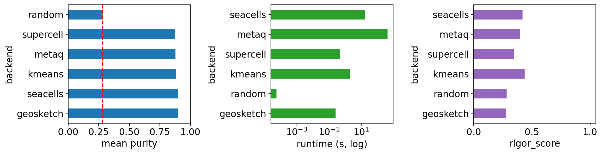
4. Rank by purity / runtime / rigor#
import matplotlib.pyplot as plt
ranked = bench.sort_values('mean_purity', ascending=True)
fig, axes = plt.subplots(1, 3, figsize=(13, 3.5))
ranked['mean_purity'].plot.barh(ax=axes[0], color='#1f77b4')
axes[0].set_xlabel('mean purity'); axes[0].set_xlim(0, 1)
axes[0].axvline(ranked['mean_purity']['random'], color='red', linestyle='--')

bench['runtime_s'].plot.barh(ax=axes[1], color='#2ca02c', logx=True)
axes[1].set_xlabel('runtime (s, log)')

bench['rigor_score'].plot.barh(ax=axes[2], color='#9467bd')
axes[2].set_xlabel('rigor_score'); axes[2].set_xlim(0, 1.05)
for ax in axes:
    ax.invert_yaxis()
plt.tight_layout(); plt.show()
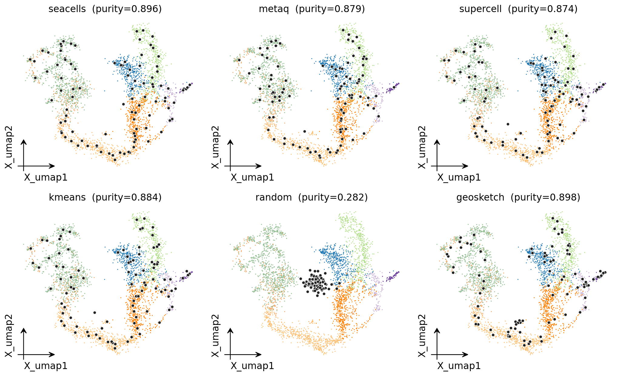
5. UMAP overlay grid#
Project all six partitions back onto the source UMAP.
# Refit each backend keeping the MetaCell object so we can use the
# ov.pl.metacell_centroids helper for each panel.
backends = ['seacells', 'metaq', 'supercell', 'kmeans', 'random', 'geosketch']
fits = {}
for b in backends:
    extra = dict(train_epoch=80, warm_epochs=10, codebook_init='random') if b == 'metaq' else {}
    fits[b] = ov.single.MetaCell(
        adata.copy(), method=b, n_metacells=100,
        use_rep='X_pca',
        device='cpu' if b != 'metaq' else 'cuda',
        random_state=0, **extra,
    ).fit()
print('refit done')
Welcome to SEACells!
Parameter graph_construction = union being used to build KNN graph...
Building kernel on X_pca
WARNING: adata.X seems to be already log-transformed.
[Epoch 1] RNA: Loss Rec=1.7653
[Epoch 1] RNA: Loss Rec=0.9919 Loss Rec Q=1.0011 | Codebook: Loss C=0.0033
[Epoch 20] RNA: Loss Rec=0.9290 Loss Rec Q=0.9383 | Codebook: Loss C=0.0076
[Epoch 40] RNA: Loss Rec=0.9147 Loss Rec Q=0.9292 | Codebook: Loss C=0.0095
[Epoch 60] RNA: Loss Rec=0.9028 Loss Rec Q=0.9254 | Codebook: Loss C=0.0095
[Epoch 80] RNA: Loss Rec=0.8912 Loss Rec Q=0.9230 | Codebook: Loss C=0.0099
refit done
fig, axes = plt.subplots(2, 3, figsize=(13, 8))
for ax, name in zip(axes.flatten(), backends):
    a = fits[name].adata
    ov.pl.embedding(a, basis='X_umap', color='clusters', ax=ax, show=False,
                    frameon='small',
                    title=f'{name}  (purity={bench.loc[name, "mean_purity"]:.3f})',
                    legend_loc=None, size=8)
    labels = fits[name]._fit_result.assignments
    pts = np.array([a.obsm['X_umap'][labels == u].mean(axis=0)
                    for u in np.unique(labels)])
    ax.scatter(pts[:, 0], pts[:, 1], s=20, c='#222',
               edgecolors='white', linewidths=0.6, zorder=5)
plt.tight_layout(); plt.show()
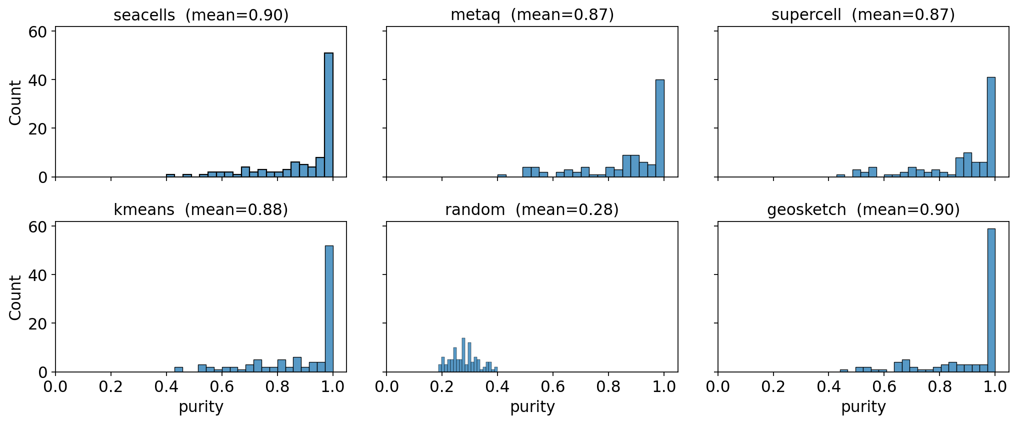
6. Purity histograms across backends#
import seaborn as sns
fig, axes = plt.subplots(2, 3, figsize=(13, 5.5), sharex=True, sharey=True)
for ax, name in zip(axes.flatten(), backends):
    p = fits[name].compute_purity('clusters')['purity']
    sns.histplot(p, bins=20, ax=ax, color='#1f77b4')
    ax.set_title(f'{name}  (mean={p.mean():.2f})')
    ax.set_xlabel('purity'); ax.set_xlim(0, 1.05)
plt.tight_layout(); plt.show()
7. Marker recovery on the aggregated AnnData#
Aggregate with each backend, then ask omicverse for the top marker per celltype in the metacell AnnData. The “right” markers (Ins1/Ins2 for Beta, Gcg for Alpha, etc.) should pop out regardless of which backend you used.
top1 = {}
for b in backends:
    ad_mc = fits[b].predicted(method='hard', layer='counts', summary='sum',
                              celltype_label='clusters')
    ad_mc = ov.pp.preprocess(ad_mc, mode='shiftlog|pearson',
                              n_HVGs=min(2000, ad_mc.n_vars))
    counts = ad_mc.obs['clusters'].value_counts()
    keep = counts[counts >= 2].index.tolist()
    ad_mc = ad_mc[ad_mc.obs['clusters'].isin(keep)].copy()
    ad_mc.obs['clusters'] = ad_mc.obs['clusters'].astype('category')
    ov.single.find_markers(ad_mc, groupby='clusters', method='wilcoxon',
                           key_added='rank_genes_groups', pts=True, use_gpu=False)
    top1[b] = pd.DataFrame(ad_mc.uns['rank_genes_groups']['names']).iloc[0]
pd.DataFrame(top1)
🔍 [2026-05-19 17:49:27] Running preprocessing in 'cpu' mode...
Begin robust gene identification
After filtration, 2000/2000 genes are kept.
Among 2000 genes, 2000 genes are robust.
✅ Robust gene identification completed successfully.
Begin size normalization: shiftlog and HVGs selection pearson
🔍 Count Normalization:
Target sum: 500000.0
Exclude highly expressed: True
Max fraction threshold: 0.2
⚠️ Excluding 1 highly-expressed genes from normalization computation
Excluded genes: ['Ghrl']
✅ Count Normalization Completed Successfully!
✓ Processed: 100 cells × 2,000 genes
✓ Runtime: 0.00s
🔍 Highly Variable Genes Selection (Experimental):
Method: pearson_residuals
Target genes: 2,000
Theta (overdispersion): 100
✅ Experimental HVG Selection Completed Successfully!
✓ Selected: 2,000 highly variable genes out of 2,000 total (100.0%)
✓ Results added to AnnData object:
• 'highly_variable': Boolean vector (adata.var)
• 'highly_variable_rank': Float vector (adata.var)
• 'highly_variable_nbatches': Int vector (adata.var)
• 'highly_variable_intersection': Boolean vector (adata.var)
• 'means': Float vector (adata.var)
• 'variances': Float vector (adata.var)
• 'residual_variances': Float vector (adata.var)
Time to analyze data in cpu: 0.10 seconds.
✅ Preprocessing completed successfully.
Added:
'highly_variable_features', boolean vector (adata.var)
'means', float vector (adata.var)
'variances', float vector (adata.var)
'residual_variances', float vector (adata.var)
'counts', raw counts layer (adata.layers)
End of size normalization: shiftlog and HVGs selection pearson
╭─ SUMMARY: preprocess ──────────────────────────────────────────────╮
│ Duration: 0.1051s │
│ Shape: 100 x 2,000 (Unchanged) │
│ │
│ CHANGES DETECTED │
│ ──────────────── │
│ ● UNS │ ✚ REFERENCE_MANU │
│ │ ✚ _ov_provenance │
│ │ ✚ history_log │
│ │ ✚ hvg │
│ │ ✚ log1p │
│ │ ✚ status │
│ │ ✚ status_args │
│ │
│ ● LAYERS │ ✚ counts (sparse matrix, 100x2000) │
│ │
╰────────────────────────────────────────────────────────────────────╯
🔍 Finding marker genes | method: wilcoxon | groupby: clusters | n_groups: 8 | n_genes: 50
✅ Done | 8 groups × 50 genes | corr: benjamini-hochberg | stored in adata.uns['rank_genes_groups']
🔍 [2026-05-19 17:49:27] Running preprocessing in 'cpu' mode...
Begin robust gene identification
After filtration, 2000/2000 genes are kept.
Among 2000 genes, 2000 genes are robust.
✅ Robust gene identification completed successfully.
Begin size normalization: shiftlog and HVGs selection pearson
🔍 Count Normalization:
Target sum: 500000.0
Exclude highly expressed: True
Max fraction threshold: 0.2
⚠️ Excluding 0 highly-expressed genes from normalization computation
Excluded genes: []
✅ Count Normalization Completed Successfully!
✓ Processed: 100 cells × 2,000 genes
✓ Runtime: 0.00s
🔍 Highly Variable Genes Selection (Experimental):
Method: pearson_residuals
Target genes: 2,000
Theta (overdispersion): 100
✅ Experimental HVG Selection Completed Successfully!
✓ Selected: 2,000 highly variable genes out of 2,000 total (100.0%)
✓ Results added to AnnData object:
• 'highly_variable': Boolean vector (adata.var)
• 'highly_variable_rank': Float vector (adata.var)
• 'highly_variable_nbatches': Int vector (adata.var)
• 'highly_variable_intersection': Boolean vector (adata.var)
• 'means': Float vector (adata.var)
• 'variances': Float vector (adata.var)
• 'residual_variances': Float vector (adata.var)
Time to analyze data in cpu: 0.02 seconds.
✅ Preprocessing completed successfully.
Added:
'highly_variable_features', boolean vector (adata.var)
'means', float vector (adata.var)
'variances', float vector (adata.var)
'residual_variances', float vector (adata.var)
'counts', raw counts layer (adata.layers)
End of size normalization: shiftlog and HVGs selection pearson
╭─ SUMMARY: preprocess ──────────────────────────────────────────────╮
│ Duration: 0.0253s │
│ Shape: 100 x 2,000 (Unchanged) │
│ │
│ CHANGES DETECTED │
│ ──────────────── │
│ ● UNS │ ✚ REFERENCE_MANU │
│ │ ✚ _ov_provenance │
│ │ ✚ history_log │
│ │ ✚ hvg │
│ │ ✚ log1p │
│ │ ✚ status │
│ │ ✚ status_args │
│ │
│ ● LAYERS │ ✚ counts (sparse matrix, 100x2000) │
│ │
╰────────────────────────────────────────────────────────────────────╯
🔍 Finding marker genes | method: wilcoxon | groupby: clusters | n_groups: 7 | n_genes: 50
✅ Done | 7 groups × 50 genes | corr: benjamini-hochberg | stored in adata.uns['rank_genes_groups']
🔍 [2026-05-19 17:49:28] Running preprocessing in 'cpu' mode...
Begin robust gene identification
After filtration, 2000/2000 genes are kept.
Among 2000 genes, 2000 genes are robust.
✅ Robust gene identification completed successfully.
Begin size normalization: shiftlog and HVGs selection pearson
🔍 Count Normalization:
Target sum: 500000.0
Exclude highly expressed: True
Max fraction threshold: 0.2
⚠️ Excluding 1 highly-expressed genes from normalization computation
Excluded genes: ['Ghrl']
✅ Count Normalization Completed Successfully!
✓ Processed: 100 cells × 2,000 genes
✓ Runtime: 0.00s
🔍 Highly Variable Genes Selection (Experimental):
Method: pearson_residuals
Target genes: 2,000
Theta (overdispersion): 100
✅ Experimental HVG Selection Completed Successfully!
✓ Selected: 2,000 highly variable genes out of 2,000 total (100.0%)
✓ Results added to AnnData object:
• 'highly_variable': Boolean vector (adata.var)
• 'highly_variable_rank': Float vector (adata.var)
• 'highly_variable_nbatches': Int vector (adata.var)
• 'highly_variable_intersection': Boolean vector (adata.var)
• 'means': Float vector (adata.var)
• 'variances': Float vector (adata.var)
• 'residual_variances': Float vector (adata.var)
Time to analyze data in cpu: 0.02 seconds.
✅ Preprocessing completed successfully.
Added:
'highly_variable_features', boolean vector (adata.var)
'means', float vector (adata.var)
'variances', float vector (adata.var)
'residual_variances', float vector (adata.var)
'counts', raw counts layer (adata.layers)
End of size normalization: shiftlog and HVGs selection pearson
╭─ SUMMARY: preprocess ──────────────────────────────────────────────╮
│ Duration: 0.0246s │
│ Shape: 100 x 2,000 (Unchanged) │
│ │
│ CHANGES DETECTED │
│ ──────────────── │
│ ● UNS │ ✚ REFERENCE_MANU │
│ │ ✚ _ov_provenance │
│ │ ✚ history_log │
│ │ ✚ hvg │
│ │ ✚ log1p │
│ │ ✚ status │
│ │ ✚ status_args │
│ │
│ ● LAYERS │ ✚ counts (sparse matrix, 100x2000) │
│ │
╰────────────────────────────────────────────────────────────────────╯
🔍 Finding marker genes | method: wilcoxon | groupby: clusters | n_groups: 8 | n_genes: 50
✅ Done | 8 groups × 50 genes | corr: benjamini-hochberg | stored in adata.uns['rank_genes_groups']
🔍 [2026-05-19 17:49:28] Running preprocessing in 'cpu' mode...
Begin robust gene identification
After filtration, 2000/2000 genes are kept.
Among 2000 genes, 2000 genes are robust.
✅ Robust gene identification completed successfully.
Begin size normalization: shiftlog and HVGs selection pearson
🔍 Count Normalization:
Target sum: 500000.0
Exclude highly expressed: True
Max fraction threshold: 0.2
⚠️ Excluding 1 highly-expressed genes from normalization computation
Excluded genes: ['Ghrl']
✅ Count Normalization Completed Successfully!
✓ Processed: 100 cells × 2,000 genes
✓ Runtime: 0.00s
🔍 Highly Variable Genes Selection (Experimental):
Method: pearson_residuals
Target genes: 2,000
Theta (overdispersion): 100
✅ Experimental HVG Selection Completed Successfully!
✓ Selected: 2,000 highly variable genes out of 2,000 total (100.0%)
✓ Results added to AnnData object:
• 'highly_variable': Boolean vector (adata.var)
• 'highly_variable_rank': Float vector (adata.var)
• 'highly_variable_nbatches': Int vector (adata.var)
• 'highly_variable_intersection': Boolean vector (adata.var)
• 'means': Float vector (adata.var)
• 'variances': Float vector (adata.var)
• 'residual_variances': Float vector (adata.var)
Time to analyze data in cpu: 0.02 seconds.
✅ Preprocessing completed successfully.
Added:
'highly_variable_features', boolean vector (adata.var)
'means', float vector (adata.var)
'variances', float vector (adata.var)
'residual_variances', float vector (adata.var)
'counts', raw counts layer (adata.layers)
End of size normalization: shiftlog and HVGs selection pearson
╭─ SUMMARY: preprocess ──────────────────────────────────────────────╮
│ Duration: 0.0252s │
│ Shape: 100 x 2,000 (Unchanged) │
│ │
│ CHANGES DETECTED │
│ ──────────────── │
│ ● UNS │ ✚ REFERENCE_MANU │
│ │ ✚ _ov_provenance │
│ │ ✚ history_log │
│ │ ✚ hvg │
│ │ ✚ log1p │
│ │ ✚ status │
│ │ ✚ status_args │
│ │
│ ● LAYERS │ ✚ counts (sparse matrix, 100x2000) │
│ │
╰────────────────────────────────────────────────────────────────────╯
🔍 Finding marker genes | method: wilcoxon | groupby: clusters | n_groups: 8 | n_genes: 50
✅ Done | 8 groups × 50 genes | corr: benjamini-hochberg | stored in adata.uns['rank_genes_groups']
🔍 [2026-05-19 17:49:28] Running preprocessing in 'cpu' mode...
Begin robust gene identification
After filtration, 2000/2000 genes are kept.
Among 2000 genes, 2000 genes are robust.
✅ Robust gene identification completed successfully.
Begin size normalization: shiftlog and HVGs selection pearson
🔍 Count Normalization:
Target sum: 500000.0
Exclude highly expressed: True
Max fraction threshold: 0.2
⚠️ Excluding 0 highly-expressed genes from normalization computation
Excluded genes: []
✅ Count Normalization Completed Successfully!
✓ Processed: 100 cells × 2,000 genes
✓ Runtime: 0.00s
🔍 Highly Variable Genes Selection (Experimental):
Method: pearson_residuals
Target genes: 2,000
Theta (overdispersion): 100
✅ Experimental HVG Selection Completed Successfully!
✓ Selected: 2,000 highly variable genes out of 2,000 total (100.0%)
✓ Results added to AnnData object:
• 'highly_variable': Boolean vector (adata.var)
• 'highly_variable_rank': Float vector (adata.var)
• 'highly_variable_nbatches': Int vector (adata.var)
• 'highly_variable_intersection': Boolean vector (adata.var)
• 'means': Float vector (adata.var)
• 'variances': Float vector (adata.var)
• 'residual_variances': Float vector (adata.var)
Time to analyze data in cpu: 0.02 seconds.
✅ Preprocessing completed successfully.
Added:
'highly_variable_features', boolean vector (adata.var)
'means', float vector (adata.var)
'variances', float vector (adata.var)
'residual_variances', float vector (adata.var)
'counts', raw counts layer (adata.layers)
End of size normalization: shiftlog and HVGs selection pearson
╭─ SUMMARY: preprocess ──────────────────────────────────────────────╮
│ Duration: 0.0276s │
│ Shape: 100 x 2,000 (Unchanged) │
│ │
│ CHANGES DETECTED │
│ ──────────────── │
│ ● UNS │ ✚ REFERENCE_MANU │
│ │ ✚ _ov_provenance │
│ │ ✚ history_log │
│ │ ✚ hvg │
│ │ ✚ log1p │
│ │ ✚ status │
│ │ ✚ status_args │
│ │
│ ● LAYERS │ ✚ counts (sparse matrix, 100x2000) │
│ │
╰────────────────────────────────────────────────────────────────────╯
🔍 Finding marker genes | method: wilcoxon | groupby: clusters | n_groups: 5 | n_genes: 50
✅ Done | 5 groups × 50 genes | corr: benjamini-hochberg | stored in adata.uns['rank_genes_groups']
🔍 [2026-05-19 17:49:28] Running preprocessing in 'cpu' mode...
Begin robust gene identification
After filtration, 2000/2000 genes are kept.
Among 2000 genes, 2000 genes are robust.
✅ Robust gene identification completed successfully.
Begin size normalization: shiftlog and HVGs selection pearson
🔍 Count Normalization:
Target sum: 500000.0
Exclude highly expressed: True
Max fraction threshold: 0.2
⚠️ Excluding 1 highly-expressed genes from normalization computation
Excluded genes: ['Ghrl']
✅ Count Normalization Completed Successfully!
✓ Processed: 100 cells × 2,000 genes
✓ Runtime: 0.00s
🔍 Highly Variable Genes Selection (Experimental):
Method: pearson_residuals
Target genes: 2,000
Theta (overdispersion): 100
✅ Experimental HVG Selection Completed Successfully!
✓ Selected: 2,000 highly variable genes out of 2,000 total (100.0%)
✓ Results added to AnnData object:
• 'highly_variable': Boolean vector (adata.var)
• 'highly_variable_rank': Float vector (adata.var)
• 'highly_variable_nbatches': Int vector (adata.var)
• 'highly_variable_intersection': Boolean vector (adata.var)
• 'means': Float vector (adata.var)
• 'variances': Float vector (adata.var)
• 'residual_variances': Float vector (adata.var)
Time to analyze data in cpu: 0.02 seconds.
✅ Preprocessing completed successfully.
Added:
'highly_variable_features', boolean vector (adata.var)
'means', float vector (adata.var)
'variances', float vector (adata.var)
'residual_variances', float vector (adata.var)
'counts', raw counts layer (adata.layers)
End of size normalization: shiftlog and HVGs selection pearson
╭─ SUMMARY: preprocess ──────────────────────────────────────────────╮
│ Duration: 0.0236s │
│ Shape: 100 x 2,000 (Unchanged) │
│ │
│ CHANGES DETECTED │
│ ──────────────── │
│ ● UNS │ ✚ REFERENCE_MANU │
│ │ ✚ _ov_provenance │
│ │ ✚ history_log │
│ │ ✚ hvg │
│ │ ✚ log1p │
│ │ ✚ status │
│ │ ✚ status_args │
│ │
│ ● LAYERS │ ✚ counts (sparse matrix, 100x2000) │
│ │
╰────────────────────────────────────────────────────────────────────╯
🔍 Finding marker genes | method: wilcoxon | groupby: clusters | n_groups: 8 | n_genes: 50
✅ Done | 8 groups × 50 genes | corr: benjamini-hochberg | stored in adata.uns['rank_genes_groups']
| seacells | metaq | supercell | kmeans | random | geosketch | |
|---|---|---|---|---|---|---|
| Alpha | Sphkap | Tmem27 | Smarca1 | Smarca1 | Irx2 | Zcchc18 |
| Beta | Gng12 | Mapt | Sytl4 | Gng12 | Sec61b | Sytl4 |
| Delta | Rbp4 | NaN | Rbp4 | Scn3a | NaN | Sst |
| Ductal | Nudt19 | Nudt19 | Lurap1l | Nudt19 | Spp1 | Hpgd |
| Epsilon | Ghrl | Guca2b | Ghrl | Gm11837 | NaN | Anpep |
| Ngn3 high EP | Numbl | Numbl | Cbfa2t3 | Cbfa2t3 | Cotl1 | Smarcd2 |
| Ngn3 low EP | Cited4 | Cat | Grin3a | Angptl4 | NaN | Atoh8 |
| Pre-endocrine | Eif3e | Cystm1 | Bax | Neat1 | Fev | Fev |
8. Recommendation table#
A rough decision tree for this kind of dataset (mid-size mouse scRNA-seq atlas, no batch / multi-modal complications):
Downstream task |
Pick |
|---|---|
UMAP / Leiden / pretty plots |
|
Differential expression / pseudobulk DESeq2 |
|
Cell–cell communication (CellPhoneDB / LIANA) |
|
Gene regulatory networks (SCENIC) |
|
Atlas with new samples arriving over time |
|
Multi-million cell dataset |
|
Quick sanity check that the pipeline works at all |
|
The most important rule: include random in your benchmark. If your
principled metacell pipeline isn’t beating random on purity / rigor, you
have a bug, not metacells.