SPATA2-inspired AnnData spatial utilities in OmicVerse

SPATA2-inspired AnnData spatial utilities in OmicVerse#

ov.space carries a small AnnData-native slice of the SPATA2 coordinate, variable, outline and outlier workflows. This notebook runs every one of those eight functions on the slide SPATA2 itself ships, so each result can be held against the R package rather than only against the notebook that produced it.

API PR: omicverse/omicverse#847
Rewrite repository: omicverse/py-SPATA2
SPATA2 documentation: theMILOlab.github.io/SPATA2
The vignette this data comes from: initiation & preprocessing, customized

This is a helper layer, not a port. The last section gives the audited coverage number so nobody reads it as one.

What this notebook covers#

Spatial task	`ov.space` function	Output
Coordinate table	`spata2_get_coords`	observation-indexed `DataFrame`
Variables beside coordinates	`spata2_extract_variables`, `spata2_join_variables`	`obs` columns and gene values in one frame
Tissue outline	`spata2_tissue_outline`	hull vertices, written to `adata.uns`
Spatially isolated spots	`spata2_identify_outliers`	boolean flag in `adata.obs`
Cleaned object	`spata2_remove_outliers`	filtered `AnnData`
Pixel scale	`spata2_pixels_to_unit`, `spata2_unit_to_pixels`	explicit distance conversion

Setup#

import numpy as np
import pandas as pd
import matplotlib.pyplot as plt
import omicverse as ov

%config InlineBackend.figure_format = 'retina'

The slide#

ov.datasets.spata2_example() returns the example_data that ships with theMILOlab/SPATA2 v3.1.4 — the object that package’s own initiation vignette is built on. Counts and coordinates are carried over unchanged from the R object’s count_mtr and coords_df.

The histology images in the source .rda are not included. They are S4 EBImage objects, which is also the reason that .rda cannot be read from Python at all and had to be converted once through R.

adata = ov.datasets.spata2_example()
adata

🔍 Downloading data to ./data/spata2_example.h5ad
✅ Download completed

AnnData object with n_obs × n_vars = 3733 × 2000
    obs: 'x', 'y', 'total_counts', 'n_genes'
    uns: 'r_tissue_outline', 'source'
    obsm: 'spatial'

src = adata.uns['source']
print(f"{src['dataset']} from {src['package']}, file {src['file']}")
print(f"{adata.n_obs:,} spots x {adata.n_vars:,} genes, {int(adata.X.sum()):,} counts")

SPATA2 example_data from theMILOlab/SPATA2 v3.1.4, file data/example_data.rda
3,733 spots x 2,000 genes, 3,494,849 counts

Coordinates#

spata2_get_coords reads adata.obsm['spatial'] and returns a tidy table. With include_obs it appends observation metadata, while protecting the three columns it owns — barcode, x, y. This slide carries its own x/y in obs, which is exactly the collision that protection exists for: the returned x and y are the coordinates, not the obs columns of the same name.

coords_df = ov.space.spata2_get_coords(adata, include_obs=['total_counts', 'n_genes'])
coords_df.head()

	barcode	x	y	total_counts	n_genes
AAACAAGTATCTCCCA-1	AAACAAGTATCTCCCA-1	434.76	226.20	566	211
AAACACCAATAACTGC-1	AAACACCAATAACTGC-1	131.76	171.24	937	369
AAACAGAGCGACTCCT-1	AAACAGAGCGACTCCT-1	407.16	454.80	902	261
AAACAGCTTTCAGAAG-1	AAACAGCTTTCAGAAG-1	96.00	273.00	1576	385
AAACAGGGTCTATATT-1	AAACAGGGTCTATATT-1	110.40	247.44	1459	416

same_as_obsm = np.allclose(coords_df[['x', 'y']].to_numpy(), adata.obsm['spatial'])
print(f"x/y came from obsm['spatial'], not from obs: {same_as_obsm}")
print(f"columns: {list(coords_df.columns)}")

x/y came from obsm['spatial'], not from obs: True
columns: ['barcode', 'x', 'y', 'total_counts', 'n_genes']

Variables beside the coordinates#

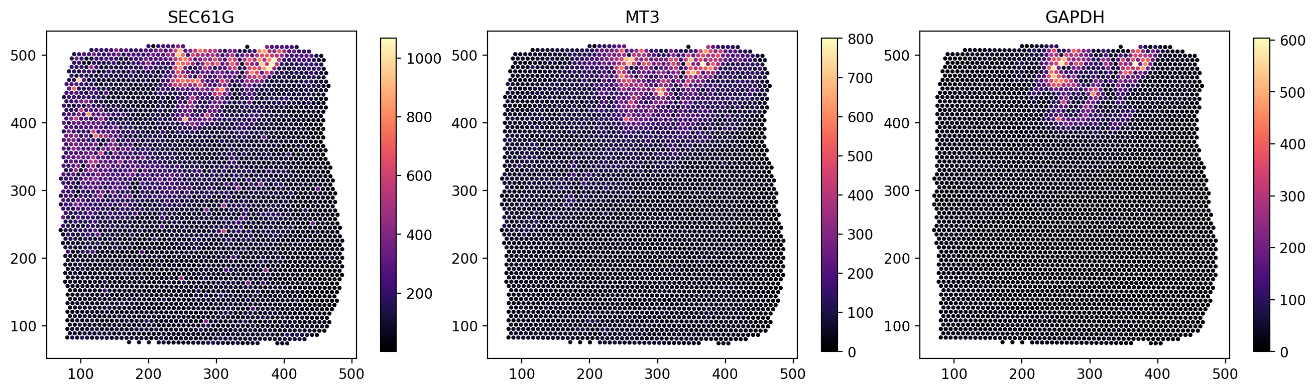
spata2_extract_variables pulls obs columns and gene expression into one frame and spata2_join_variables puts that frame next to the coordinates, which is the shape most spatial plotting wants.

top_genes = adata.var_names[np.asarray(adata.X.sum(axis=0)).ravel().argsort()[::-1][:3]]
feature_df = ov.space.spata2_join_variables(adata, list(top_genes) + ['total_counts'])
print(f"three most-expressed genes: {list(top_genes)}")
feature_df.head()

three most-expressed genes: ['SEC61G', 'MT3', 'GAPDH']

	barcode	x	y	SEC61G	MT3	GAPDH	total_counts
AAACAAGTATCTCCCA-1	AAACAAGTATCTCCCA-1	434.76	226.20	151	28	6	566
AAACACCAATAACTGC-1	AAACACCAATAACTGC-1	131.76	171.24	62	55	23	937
AAACAGAGCGACTCCT-1	AAACAGAGCGACTCCT-1	407.16	454.80	111	114	23	902
AAACAGCTTTCAGAAG-1	AAACAGCTTTCAGAAG-1	96.00	273.00	280	77	21	1576
AAACAGGGTCTATATT-1	AAACAGGGTCTATATT-1	110.40	247.44	201	90	31	1459

fig, axes = plt.subplots(1, 3, figsize=(13, 4), constrained_layout=True)
for ax, gene in zip(axes, top_genes):
    s = ax.scatter(feature_df['x'], feature_df['y'], c=feature_df[gene], s=4, cmap='magma')
    ax.set_title(gene); ax.set_aspect('equal'); fig.colorbar(s, ax=ax, shrink=0.8)
plt.show()

../_images/3579f37d39659f971d99fd9ea1fcfe151c408962b0b3eb5d781a7c809cd345f7.png

Tissue outline#

spata2_tissue_outline returns a convex hull of the spots and writes it to adata.uns.

SPATA2’s identifyTissueOutline(method = "obs") does something different: it runs concaveman(concavity = 2), and separately assigns every spot a tissue_section with DBSCAN so a slide carrying several fragments produces one outline per fragment. The dataset carries SPATA2’s own answer in adata.uns['r_tissue_outline'] — the vertices concaveman::concaveman(concavity = 2) produced under R 4.4 on these exact coordinates — so the two can be laid over each other here without needing R.

outline = ov.space.spata2_tissue_outline(adata)
r_outline = adata.uns['r_tissue_outline']
print(f"ov.space convex hull: {len(outline)} vertices")
print(f"R SPATA2 concaveman : {len(r_outline)} vertices")
print(f"written to adata.uns: {[k for k in adata.uns if 'outline' in k]}")

ov.space convex hull: 34 vertices
R SPATA2 concaveman : 170 vertices
written to adata.uns: ['r_tissue_outline', 'spata2_tissue_outline', 'spata2_tissue_outline_source_obs']

def polygon_area(pts):
    x, y = np.asarray(pts)[:, 0], np.asarray(pts)[:, 1]
    return 0.5 * abs(np.dot(x, np.roll(y, 1)) - np.dot(y, np.roll(x, 1)))

a_convex, a_concave = polygon_area(outline[['x', 'y']]), polygon_area(r_outline)
print(f"convex hull area   {a_convex:12,.1f}")
print(f"SPATA2 outline area{a_concave:12,.1f}")
print(f"the convex hull is {a_convex / a_concave:.3f}x the tissue SPATA2 outlines")

convex hull area      173,041.8
SPATA2 outline area   168,821.6
the convex hull is 1.025x the tissue SPATA2 outlines

def compare_outlines(spatial, r_pts, py_pts):
    ring = lambda p: np.vstack([np.asarray(p, float), np.asarray(p, float)[:1]])
    fig, ax = plt.subplots(figsize=(6.5, 6.5))
    ax.scatter(spatial[:, 0], spatial[:, 1], s=3, c='#d0d0d0')
    ax.plot(*ring(r_pts).T, lw=2.4, c='#d62728', label='R SPATA2 concaveman(2)')
    ax.plot(*ring(py_pts).T, lw=1.8, c='#1f77b4', ls='--', label='ov.space convex hull')
    ax.set_aspect('equal')
    ax.legend(loc='lower left')
    return ax

compare_outlines(adata.obsm['spatial'], r_outline, outline[['x', 'y']].to_numpy())
plt.show()

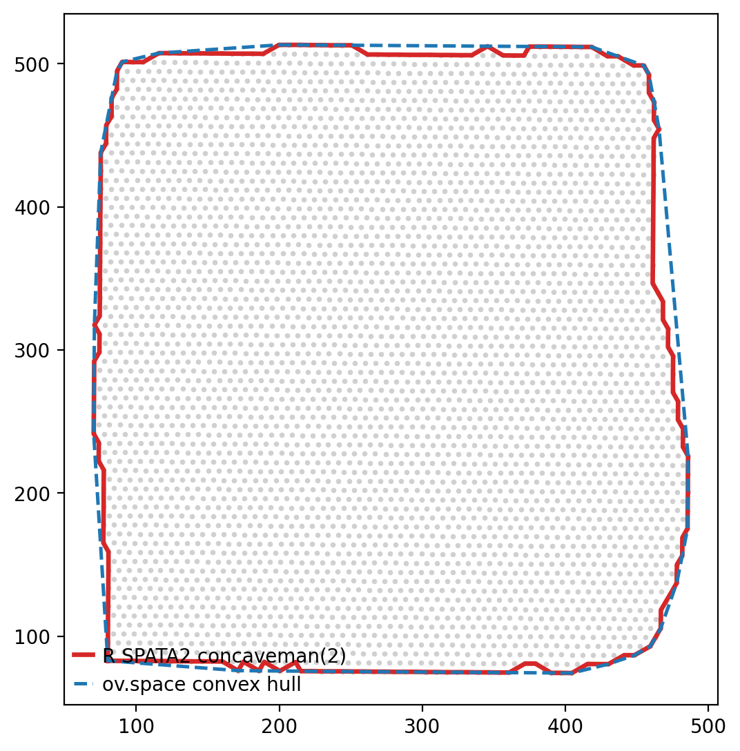
../_images/68065d890cefd5375b98897508d6247b568253d0f8aa4f8765b1c548c042e70b.png

The two track each other closely on this slide, because the spots fill the capture area and the point cloud is already near-convex. Measured on a second real slide as well:

slide	spots	convex	concaveman(2)	ratio
SPATA2 `example_data`	3,733	173,041.8	168,821.6	1.025
DLPFC 151673	4,910	316,686,266	316,430,828	1.001

DBSCAN finds a single tissue section and no noise spots in both, so the per-section decomposition would have changed nothing either. Do not carry that conclusion to a slide whose tissue is genuinely concave, or that holds more than one fragment: a convex hull bridges the opening and merges the fragments.

Spatially isolated spots#

spata2_identify_outliers defaults to method='dbscan' — the rule SPATA2 applies in identifyTissueOutline(method = "obs"), with eps at 1.25x the centre-to-centre spot distance. Density connectivity is transitive, so a spot at the rim of the tissue stays attached to the section through its neighbours.

flags = ov.space.spata2_identify_outliers(adata)
print(f"flagged {int(flags.sum())} of {adata.n_obs:,} spots")

flagged 0 of 3,733 spots

Zero, which is the right answer for an intact section that fills its capture area.

That is worth checking rather than assuming, so plant five spots well off the tissue and confirm the rule finds exactly those and nothing else.

import anndata as ad
far = adata.obsm['spatial'].max(axis=0) + np.array([[80., 80.], [95., 70.],
                                                    [110., 90.], [70., 105.], [130., 60.]])
probe = ad.AnnData(np.zeros((adata.n_obs + 5, 1), dtype=np.float32))
probe.obsm['spatial'] = np.vstack([adata.obsm['spatial'], far])

probe_flags = ov.space.spata2_identify_outliers(probe, write_key=None).to_numpy()
print(f"flagged in total          : {int(probe_flags.sum())}")
print(f"of the five planted spots : {int(probe_flags[-5:].sum())}")
print(f"false positives elsewhere : {int(probe_flags[:-5].sum())}")

flagged in total          : 5
of the five planted spots : 5
false positives elsewhere : 0

method='mad' keeps the older rule — flag a spot whose k-th neighbour is further than a median/MAD threshold. It is not the default, and this slide is why. Spots sit on a regular lattice, so every interior spot has the same k-th neighbour distance and the deviation is zero in exact arithmetic but ~1e-14 in floating point. An earlier version tested mad == 0, which never fired; the threshold collapsed onto the median and 880 of these 3,733 spots came back flagged, all of them intact tissue. spata2_remove_outliers would have deleted a quarter of the section.

That guard is now a relative tolerance, but the rule still has no power on a lattice — once the spread is genuinely degenerate nothing can exceed the threshold. Keep it for irregularly sampled coordinates.

mad_flags = ov.space.spata2_identify_outliers(probe, method='mad', write_key=None)
print(f"method='mad' on the same probe: {int(mad_flags.sum())} flagged "
      f"({int(mad_flags.to_numpy()[-5:].sum())} of the five planted)")

method='mad' on the same probe: 0 flagged (0 of the five planted)

Removing them#

spata2_remove_outliers drops whatever was flagged. On this slide nothing is, so the object comes back whole — which is the point.

kept = ov.space.spata2_remove_outliers(adata, copy=True)
print(f"{adata.n_obs:,} spots in, {kept.n_obs:,} out")

3,733 spots in, 3,733 out

probe_kept = ov.space.spata2_remove_outliers(probe, copy=True)
print(f"the probe with five planted spots: {probe.n_obs:,} in, {probe_kept.n_obs:,} out")

the probe with five planted spots: 3,738 in, 3,733 out

Pixel scale#

Coordinates here are pixels of the source image. spata2_pixels_to_unit and spata2_unit_to_pixels make the conversion explicit rather than leaving a bare factor in the analysis, and are exact inverses.

pixels_per_unit = 2.5
step = np.median(np.linalg.norm(np.diff(np.sort(adata.obsm['spatial'][:, 0])), axis=0))
distances = np.array([0.0, 55.0, 110.0, 220.0])
units = ov.space.spata2_pixels_to_unit(distances, pixels_per_unit=pixels_per_unit)
pd.DataFrame({'pixels': distances, 'units': units})

	pixels	units
0	0.0	0.0
1	55.0	22.0
2	110.0	44.0
3	220.0	88.0

back = ov.space.spata2_unit_to_pixels(units, pixels_per_unit=pixels_per_unit)
print(f"round-trip exact: {np.array_equal(back, distances)}")

round-trip exact: True

Timing on this slide#

import time

def timed(label, call):
    start = time.perf_counter()
    result = call()
    return {'operation': label, 'seconds': round(time.perf_counter() - start, 4),
            'shape': getattr(result, 'shape', (len(result),))}

rows = [
    timed('spata2_get_coords', lambda: ov.space.spata2_get_coords(adata)),
    timed('spata2_extract_variables', lambda: ov.space.spata2_extract_variables(adata, list(top_genes))),
    timed('spata2_join_variables', lambda: ov.space.spata2_join_variables(adata, list(top_genes))),
    timed('spata2_tissue_outline', lambda: ov.space.spata2_tissue_outline(adata, write_key=None)),
    timed('spata2_identify_outliers', lambda: ov.space.spata2_identify_outliers(adata, write_key=None)),
]
pd.DataFrame(rows)

	operation	seconds	shape
0	spata2_get_coords	0.0004	(3733, 3)
1	spata2_extract_variables	0.0043	(3733, 3)
2	spata2_join_variables	0.0045	(3733, 6)
3	spata2_tissue_outline	0.0022	(34, 2)
4	spata2_identify_outliers	0.0129	(3733,)

How much of SPATA2 this is#

The rewrite repository audits the real SPATA2 3.1.4 NAMESPACE, not a hand-picked subset: a symbol counts as implemented only when Python exposes the same R export name. Full tables in NAMESPACE_PARITY.md and spata2_namespace_parity.csv.

pd.DataFrame(
    [['R exports audited from the SPATA2 3.1.4 NAMESPACE', '751'],
     ['R-compatible Python symbols in py-SPATA2', '16'],
     ['strict namespace coverage', '2.1%'],
     ['ov.space functions exercised in this notebook', '8']],
    columns=['metric', 'value'],
)

	metric	value
0	R exports audited from the SPATA2 3.1.4 NAMESPACE	751
1	R-compatible Python symbols in py-SPATA2	16
2	strict namespace coverage	2.1%
3	ov.space functions exercised in this notebook	8

What to take from this#

These helpers are good for coordinate inspection, variable tables, a quick tissue boundary and isolated-spot filtering on AnnData. Two things this notebook established that are worth carrying forward:

the outline is convex, and on a slide that fills its capture area that is within 2.5% of what SPATA2 draws — but a concave tissue or a multi-fragment slide is a different story, and neither slide tested here is one;
the outlier rule is DBSCAN density connectivity because the median/MAD rule cannot work on a lattice; that was not visible until the helpers were run on a real slide rather than on constructed coordinates.

Coverage against the audited SPATA2 export surface is 2.1%. Treat this as a utility layer, not a port.