Lipidomics — the lipidr workflow in omicverse

Lipidomics has enough structure to deserve a dedicated analysis path. Every lipid follows the LIPID MAPS shorthand (PE 34:1, TAG 54:3, Cer d18:1/24:0), targeted assays report several transitions per lipid, and the biology is organised by class, chain length and unsaturation — none of which a generic metabolomics pipeline exploits.

omicverse integrates the Bioconductor lipidr workflow through the pure-Python pylipidr backend. Every step is a registered ov.metabol function and every object is a plain AnnData, so lipidomics drops straight into the rest of omicverse.

Pipeline. read_skyline → add_sample_annotation → summarize_transitions → annotate_lipids → normalize_pqn → de_lipids → lsea / lipid_mva.

Install the backend with pip install omicverse[lipidomics].

import matplotlib.pyplot as plt
import numpy as np
import pandas as pd

import omicverse as ov

ov.plot_set()

🔬 Starting plot initialization...
🧬 Detecting GPU devices…
🚫 No GPU devices found (CUDA/MPS/ROCm/XPU)

   ____            _     _    __                  
  / __ \____ ___  (_)___| |  / /__  _____________ 
 / / / / __ `__ \/ / ___/ | / / _ \/ ___/ ___/ _ \ 
/ /_/ / / / / / / / /__ | |/ /  __/ /  (__  )  __/ 
\____/_/ /_/ /_/_/\___/ |___/\___/_/  /____/\___/                                              

🔖 Version: 2.2.1rc1   📚 Tutorials: https://omicverse.readthedocs.io/
✅ plot_set complete.

1 — Download a raw Skyline dataset

We use lipidr’s own targeted-lipidomics example — a mouse diet study (Salek/Mohamed): liver lipids measured by LC-MS/MS, exported from Skyline. Two MIT-licensed files live on GitHub, so nothing is bundled locally:

• A1_data.csv — the long Skyline transition table (one row per transition)

• clin.csv — sample metadata: group, Diet (Normal / HighFat), BileAcid

ov.datasets.download_data caches each file under ./metabol_data.

base = 'https://raw.githubusercontent.com/ahmohamed/lipidr/master/inst/extdata'
skyline_path = ov.datasets.download_data(
    url=f'{base}/A1_data.csv', file_path='A1_data.csv', dir='./metabol_data',
)
clin_path = ov.datasets.download_data(
    url=f'{base}/clin.csv', file_path='clin.csv', dir='./metabol_data',
)

🔍 Downloading data to ./metabol_data/A1_data.csv
⚠️ File ./metabol_data/A1_data.csv already exists
🔍 Downloading data to ./metabol_data/clin.csv
⚠️ File ./metabol_data/clin.csv already exists

2 — Read the Skyline export

ov.metabol.read_skyline pivots the long transition table into an AnnData (samples × transitions). ov.metabol.add_sample_annotation joins the clinical table onto adata.obs by sample id.

adata = ov.metabol.read_skyline(skyline_path)
adata = ov.metabol.add_sample_annotation(adata, clin_path)
print(adata)
print('groups:', adata.obs['group'].value_counts().to_dict())

AnnData object with n_obs × n_vars = 58 × 102
    obs: 'group', 'Diet', 'BileAcid'
    var: 'Molecule', 'TransitionId', 'Class_skyline', 'Class', 'Category', 'total_cl', 'total_cs', 'chains', 'not_parsed', 'istd'
    uns: 'lipidr_default_measure', 'lipidr_state'
groups: {'QC': 12, 'NormalDiet_water': 11, 'NormalDiet_DCA': 11, 'HighFat_water': 11, 'HighFat_DCA': 11, 'blank': 2}

3 — Summarize transitions

A targeted assay records several transitions per lipid (different product ions). summarize_transitions collapses them to one value per lipid — method='max' keeps the most intense transition, the lipidr default and the most robust choice for quantification.

adata = ov.metabol.summarize_transitions(adata, method='max')
print('after summarization:', adata.shape, '(samples × lipids)')

after summarization: (58, 101) (samples × lipids)

4 — Annotate lipids with Goslin

ov.metabol.annotate_lipids parses every lipid name with the Goslin reference engine (pygoslin) and writes lipid_class, lipid_category, total_carbons, total_db and lipid_backbone into adata.var. Goslin understands the LIPID MAPS shorthand and the common vendor dialects, so ether lipids (PE-O, PE-P) and sphingolipids parse correctly.

adata = ov.metabol.annotate_lipids(adata)
print('lipid classes:')
print(adata.var['lipid_class'].value_counts())

lipid classes:
lipid_class
PE      25
PI      22
PE-O    18
PE-P    18
PG      11
PI-P     1
Name: count, dtype: int64

5 — Normalize with PQN

normalize_pqn applies Probabilistic Quotient Normalization: each sample is scaled by the median quotient of its lipids against a reference profile — robust to a few highly variable species. exclude='blank' drops the solvent blanks before building the reference, and log=True returns a log2 matrix ready for linear modelling.

norm = ov.metabol.normalize_pqn(adata, measure='Area', exclude='blank', log=True)
print('normalized:', norm.shape, '(blanks dropped)')
print(f'log2 intensity range: {norm.X.min():.1f} .. {norm.X.max():.1f}')

normalized: (56, 101) (blanks dropped)
log2 intensity range: 5.7 .. 23.7

6 — Differential analysis

ov.metabol.de_lipids runs limma moderated-t — the small-sample workhorse that borrows variance across lipids, far more powerful than a per-lipid t-test at n ≈ 11/group. We contrast a high-fat vs normal diet (both on water). The result table carries lipid-class annotations, which lsea needs downstream.

de = ov.metabol.de_lipids(
    norm, 'HighFat_water - NormalDiet_water', group_col='group',
)
n_sig = int((de['adj.P.Val'] < 0.05).sum())
print(f'{n_sig} / {len(de)} lipids differential at adj.P < 0.05')
de.sort_values('P.Value').head()[
    ['Molecule', 'Class', 'logFC', 'P.Value', 'adj.P.Val']]

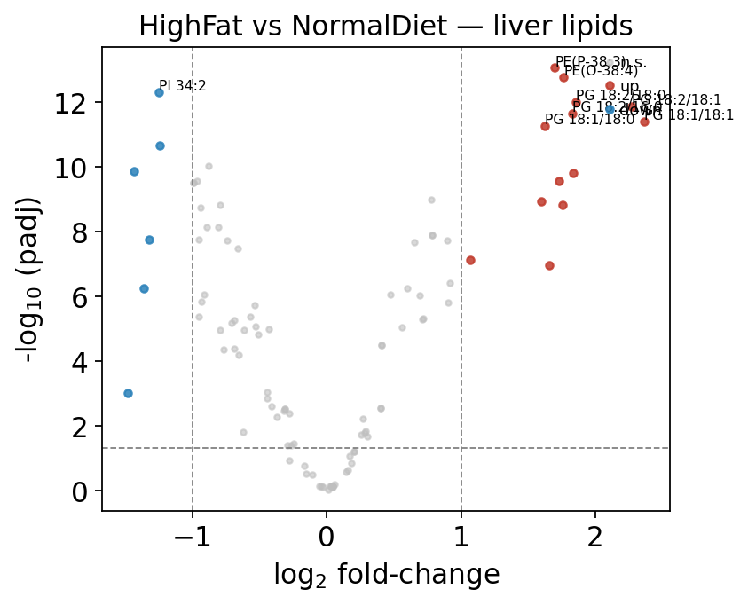
79 / 101 lipids differential at adj.P < 0.05

	Molecule	Class	logFC	P.Value	adj.P.Val
0	PE(P-38:3)	PE	1.699273	8.614843e-16	8.700992e-14
1	PE(O-38:4)	PE	1.765957	3.418962e-15	1.726576e-13
2	PI 34:2	PI	-1.252535	1.469847e-14	4.948485e-13
3	PG 18:2/18:0	PG	1.855818	4.051081e-14	1.022898e-12
4	PG 18:2/18:1	PG	2.271831	6.715486e-14	1.356528e-12

A diet swap remodels the liver lipidome wholesale, so most lipids move — exactly the regime moderated-t was built for. The volcano below uses ov.metabol.volcano; we rename the lipidr-style columns to the generic log2fc / pvalue / padj that omicverse plotting expects.

deg = de.rename(columns={
    'logFC': 'log2fc', 'P.Value': 'pvalue', 'adj.P.Val': 'padj',
}).set_index('Molecule')
fig, ax = ov.metabol.volcano(deg, padj_thresh=0.05, log2fc_thresh=1.0,
                             label_top_n=8)
ax.set_title('HighFat vs NormalDiet — liver lipids')
plt.tight_layout(); plt.show()

7 — Lipid Set Enrichment Analysis

ov.metabol.lsea runs a preranked GSEA over lipid sets built automatically from class, total chain length and total unsaturation — it answers “which lipid groups move coherently?” rather than testing species one by one. Sets are ranked by enrichment score (ES).

enr = ov.metabol.lsea(de, rank_by='logFC', nperm=2000)
enr.sort_values('pval').head(10)[
    ['set', 'ES', 'NES', 'pval', 'padj', 'size']]

	set	ES	NES	pval	padj	size
0	Class_PG	0.966667	2.381726	0.000846	0.015228	11
1	Class_PI	-0.619609	-2.047305	0.003012	0.027108	23
2	total_cs_4	0.705023	1.714467	0.012584	0.075503	10
3	total_cl_34	-0.489244	-1.525266	0.040059	0.180267	19
4	total_cl_36	0.476344	1.450170	0.050439	0.181579	29
5	total_cl_32	-0.593723	-1.429414	0.093516	0.246663	8
6	total_cl_18	0.868687	1.326131	0.108213	0.246663	2
7	Class_SPH	0.868687	1.325317	0.109628	0.246663	2
8	total_cs_2	-0.358807	-1.123383	0.273115	0.546230	18
9	total_cs_3	-0.359576	-1.049363	0.377868	0.672516	14

8 — Acyl-chain map

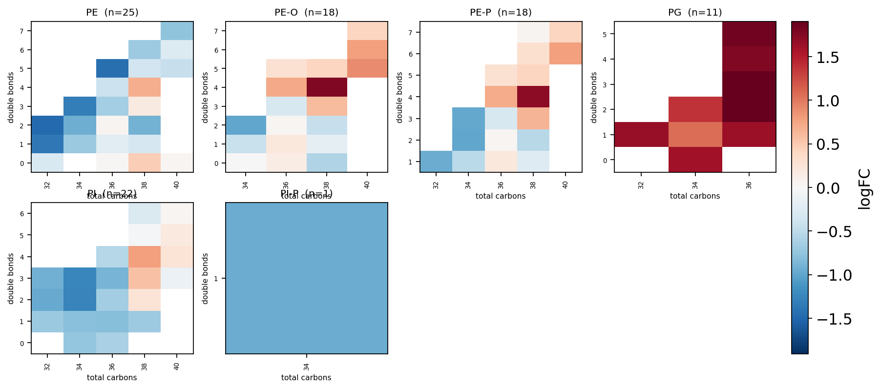
The signature lipidomics figure: a carbon × double-bond grid per class, each cell coloured by the differential statistic. It exposes trends a volcano hides — e.g. whether a class shifts toward longer or more unsaturated chains. ov.metabol.acyl_chain_map parses every lipid name and lays out one heatmap panel per class.

fig = ov.metabol.acyl_chain_map(
    de.set_index('Molecule'), value_col='logFC', n_cols=4,
)
plt.show()

9 — Multivariate analysis

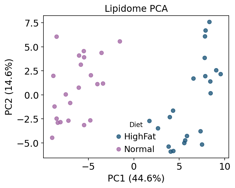
ov.metabol.lipid_mva provides PCA / PCoA / OPLS-DA on the lipid matrix. PCA on the biological samples (QC dropped) shows how strongly the two diets separate. The score plot below colours samples by Diet.

bio = norm[norm.obs['group'] != 'QC'].copy()
mva = ov.metabol.lipid_mva(bio, method='PCA', group_col='Diet')
print('explained variance:', np.round(mva.explained_variance[:3], 3))

explained variance: [0.446 0.146 0.102]

scores = mva.scores
diet = bio.obs['Diet'].reindex(scores.index).astype(str)
fig, ax = plt.subplots(figsize=(5, 4.2))
for g in sorted(diet.unique()):
    m = (diet == g).to_numpy()
    ax.scatter(scores.iloc[m, 0], scores.iloc[m, 1], label=g, s=34, alpha=0.8)
ax.set_xlabel(f'PC1 ({mva.explained_variance[0] * 100:.1f}%)')
ax.set_ylabel(f'PC2 ({mva.explained_variance[1] * 100:.1f}%)')
ax.legend(title='Diet', frameon=False); ax.set_title('Lipidome PCA')
plt.tight_layout(); plt.show()

10 — Class-level composition

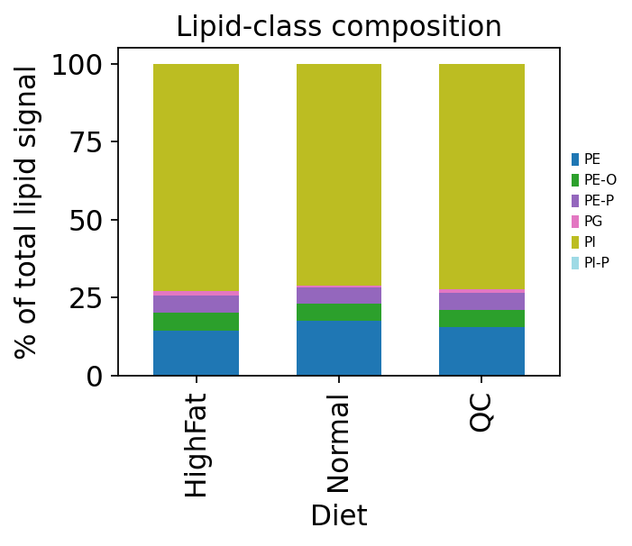
For a quick whole-lipidome overview, ov.metabol.aggregate_by_class collapses the species matrix to per-class totals. A stacked bar of the mean composition per group is the first plot most lipidomics papers show.

no_blank = adata[adata.obs['group'] != 'blank']
cls = ov.metabol.aggregate_by_class(no_blank, agg='sum')
cls.obs = no_blank.obs
print('class-level matrix:', cls.shape)
cls.var

class-level matrix: (56, 6)

	n_species
PE	25
PE-O	18
PE-P	18
PG	11
PI	22
PI-P	1

comp = pd.DataFrame(cls.X, index=cls.obs_names, columns=cls.var_names)
comp['Diet'] = cls.obs['Diet'].values
pct = comp.groupby('Diet').mean().T
pct = pct.div(pct.sum(axis=0), axis=1) * 100
fig, ax = plt.subplots(figsize=(4.6, 4))
pct.T.plot(kind='bar', stacked=True, ax=ax, colormap='tab20', width=0.6)
ax.set_ylabel('% of total lipid signal'); ax.set_xlabel('Diet')
ax.legend(loc='center left', bbox_to_anchor=(1.01, 0.5), frameon=False,
          fontsize=7)
ax.set_title('Lipid-class composition')
plt.tight_layout(); plt.show()

Summary

A complete lipidomics analysis, all AnnData-native:

Step	ov.metabol function	What it does
Import	read_skyline	Skyline export → AnnData
Metadata	add_sample_annotation	join clinical table
Collapse	summarize_transitions	transitions → one value per lipid
Annotate	annotate_lipids	Goslin class / category / chains
Normalize	normalize_pqn · normalize_istd	PQN / internal-standard
Differential	de_lipids	limma moderated-t
Enrichment	lsea · lion_enrichment	lipid-set GSEA · LION ORA
Multivariate	lipid_mva	PCA / PCoA / OPLS-DA
Visualize	volcano · acyl_chain_map · aggregate_by_class

The analysis engine is the standalone, R-parity-tested pylipidr port of Bioconductor lipidr; ov.metabol exposes it as registered functions so lipidomics composes with every other omicverse module.