ov.synbio III — CRISPR editing & directed-evolution libraries

A focused tour of two synbio workflows that ov.synbio supports end-to-end:

1. CRISPR editing — design guide RNAs for a gene, screen their specificity, and plan base edits / HDR knock-ins.

2. Directed evolution — design mutant libraries (degenerate codons, DMS) and let a protein language model guide which variants to build.

We work on a real protein — the 56-residue GB1 domain — and use ov.synbio itself to turn it into a gene, so the whole notebook is self-contained. The CRISPR/library parts are CPU-only; the model-guided step uses ESM (GPU when available).

pip install 'omicverse[synbio]'.

import omicverse as ov

ov.plot_set()
print('omicverse', ov.__version__)

🔬 Starting plot initialization...
🧬 Detecting GPU devices…
✅ NVIDIA CUDA GPUs detected: 1
    • [CUDA 0] NVIDIA H100 80GB HBM3
      Memory: 79.1 GB | Compute: 9.0

   ____            _     _    __                  
  / __ \____ ___  (_)___| |  / /__  _____________ 
 / / / / __ `__ \/ / ___/ | / / _ \/ ___/ ___/ _ \ 
/ /_/ / / / / / / / /__ | |/ /  __/ /  (__  )  __/ 
\____/_/ /_/ /_/_/\___/ |___/\___/_/  /____/\___/                                              

🔖 Version: 2.2.1rc1   📚 Tutorials: https://omicverse.readthedocs.io/
✅ plot_set complete.

omicverse 2.2.1rc1

First, turn the GB1 protein into a codon-optimized E. coli gene — this is the DNA we will target with CRISPR.

GB1 = 'MTYKLILNGKTLKGETTTEAVDAATAEKVFKQYANDNGVDGEWTYDDATKTFTVTE'
gene = ov.synbio.codon_optimize(GB1, host='e_coli').sequence
print('gene length:', len(gene), 'bp')
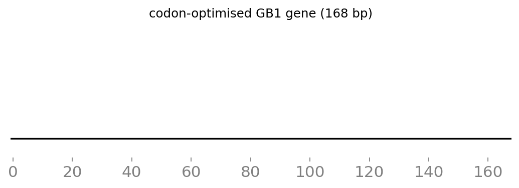
ov.synbio.view_construct(gene, title='codon-optimised GB1 gene')   # the CRISPR target, as a map
None

gene length: 168 bp

1 — Guide-RNA design

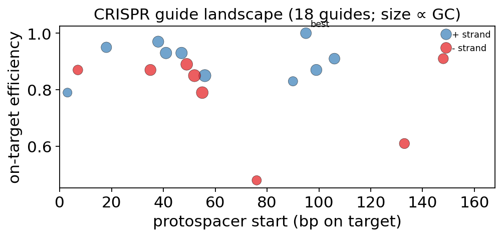
design_grnas scans both strands for SpCas9 NGG PAM sites, extracts 20-nt protospacers, filters on GC, and ranks them by an on-target efficiency heuristic (GC, poly-T terminators, PAM-proximal G).

guides = ov.synbio.design_grnas(gene, enzyme='SpCas9')
print(f'{len(guides)} candidate guides; best 3:')
for g in guides[:3]:
    print(' ', g)

18 candidate guides; best 3:
  Guide(GTATGCGAACGATAACGGCG TGG +@95 GC=0.55 eff=1.00)
  Guide(AGGCGAAACCACCACCGAAG CGG +@38 GC=0.60 eff=0.97)
  Guide(CTGAACGGCAAAACCCTGAA AGG +@18 GC=0.50 eff=0.95)

Compare algorithms. The ranking above uses method='heuristic' (GC / poly-T rules). method='rs3' scores each guide with the real Rule Set 3 model (DeWeirdt 2021) — the maintained successor to Azimuth / Rule Set 2 — which can re-rank the guides based on the trained on-target model.

# on-target: heuristic vs the REAL Rule Set 3 model (Azimuth's successor) — side by side
flanked = 'GCATGCATGC' + gene + 'GCATGCATGC'    # flanks so guides get a full 30-mer context
gh = ov.synbio.design_grnas(flanked, method='heuristic')
gr = ov.synbio.design_grnas(flanked, method='rs3')
print(f"heuristic top: {gh[0].spacer} score={gh[0].efficiency:.2f}")
print(f"rs3 (real) top: {gr[0].spacer} score={gr[0].efficiency:.2f}  (Rule Set 3 z-score)")
# the real Rule Set 3 landscape along the gene (efficiency = trained-model score)
ov.synbio.plot_grna_efficiency(gr, target_len=len(flanked))
None

Calculating sequence-based features
heuristic top: GTATGCGAACGATAACGGCG score=1.00
rs3 (real) top: GTATGCGAACGATAACGGCG score=1.07  (Rule Set 3 z-score)

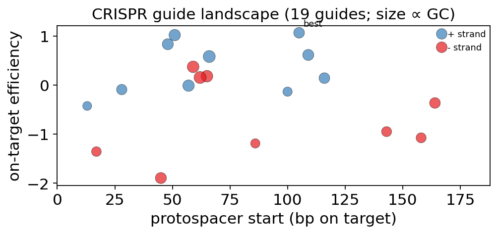
plot_grna_efficiency maps the candidates along the gene — position vs efficiency, coloured by strand, sized by GC — so you can pick a well-placed, efficient guide.

ov.synbio.plot_grna_efficiency(guides, target_len=len(gene))
None

2 — Off-target specificity

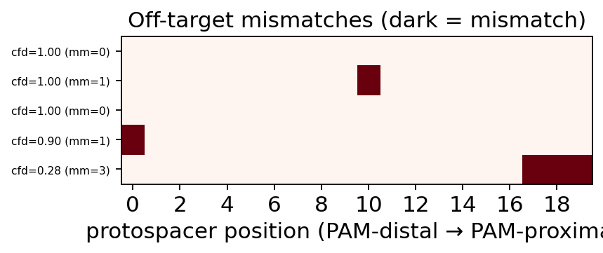
A guide is only useful if it’s specific. offtarget_search finds near-matches (here in a synthetic background carrying a few decoy sites) and scores them with a seed-weighted, CFD-style model — mismatches in the PAM-proximal seed hurt far more than distal ones.

spacer = guides[0].spacer
# build a background with the on-target plus 3 decoys carrying 1-3 seed/distal mismatches
decoys = [spacer, 'A' + spacer[1:], spacer[:10] + 'AA' + spacer[12:], spacer[:-3] + 'AAA']
background = 'GC'.join(d + 'TGG' for d in decoys) + gene
offs = ov.synbio.offtarget_search(spacer, background, max_mismatches=4)
print(f'{len(offs)} sites; top:')
for o in offs[:4]:
    print(' ', o)

5 sites; top:
  OffTarget(@0+ mm=0 cfd=1.000)
  OffTarget(@50+ mm=1 cfd=1.000)
  OffTarget(@193+ mm=0 cfd=1.000)
  OffTarget(@25+ mm=1 cfd=0.900)

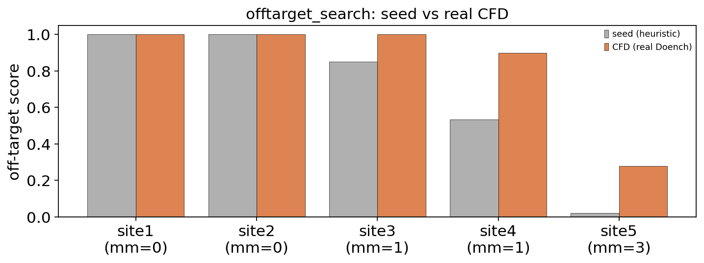
Compare algorithms. method='seed' is a dependency-free seed-weighted approximation; method='cfd' (the default) uses the real Doench-2016 CFD tables (240 empirically-measured mismatch factors, vendored from CRISPOR). Note how a PAM-proximal (seed) mismatch is scored very differently by the calibrated CFD.

# off-target: seed heuristic vs the REAL Doench-2016 CFD tables — side by side
seed = ov.synbio.offtarget_search(spacer, background, method='seed')
cfd  = ov.synbio.offtarget_search(spacer, background, method='cfd')
labels, sv, cv = [], [], []
for i, (s, c) in enumerate(zip(seed, cfd)):
    print(f"  mm={s.mismatches}  seed={s.cfd:.3f}   CFD(real Doench)={c.cfd:.3f}")
    labels.append(f"site{i+1}\n(mm={s.mismatches})"); sv.append(s.cfd); cv.append(c.cfd)
ov.synbio.plot_method_comparison(labels, {'seed (heuristic)': sv, 'CFD (real Doench)': cv},
    ylabel='off-target score', title='offtarget_search: seed vs real CFD')
None

mm=0  seed=1.000   CFD(real Doench)=1.000
  mm=0  seed=1.000   CFD(real Doench)=1.000
  mm=1  seed=0.850   CFD(real Doench)=1.000
  mm=1  seed=0.534   CFD(real Doench)=0.900
  mm=3  seed=0.022   CFD(real Doench)=0.278

plot_offtargets draws the mismatch matrix — one row per candidate site (ranked by CFD), dark cells where the site differs from the guide. A row with only PAM-distal (left) mismatches is more dangerous than one with seed (right) mismatches.

ov.synbio.plot_offtargets(offs, spacer=spacer)
None

3 — Base editing & HDR knock-in

Beyond cutting: base_editor_window reports which bases an adenine or cytosine base editor could change within its activity window (protospacer positions 4–8), and hdr_arms builds a homology-directed-repair donor to insert a payload at the cut site.

print('ABE (A->G):', ov.synbio.base_editor_window(spacer, editor='ABE'))
donor = ov.synbio.hdr_arms(gene, cut_site=len(gene)//2, arm_length=30, insert='CATCATCATCACCATCAC')  # 6xHis
print('HDR donor:', donor['left_len'], 'bp + 6xHis insert +', donor['right_len'], 'bp')

ABE (A->G): {'editor': 'ABE', 'window': (4, 8), 'target_base': 'A', 'n_edits': 1, 'edits': [{'position': 8, 'from': 'A', 'to': 'G'}], 'edited_spacer': 'GTATGCGGACGATAACGGCG'}
HDR donor: 30 bp + 6xHis insert + 30 bp

4 — Mutant-library design

To evolve a protein you screen a library. degenerate_codon finds the minimal IUPAC codon covering a desired amino-acid set (all 20 → NNK/NNS, with no wasted codons), and saturation_library / dms_library size the experiment.

print('all 20 AA ->', ov.synbio.degenerate_codon(list('ACDEFGHIKLMNPQRSTVWY')))
print('small+polar (A,S,T,G) ->', ov.synbio.degenerate_codon(['A', 'S', 'T', 'G']))
print('3-site NNK saturation:', ov.synbio.saturation_library(3, 'NNK'))
lib = ov.synbio.dms_library(GB1, positions=[3, 5, 27])
print('DMS at 3 positions:', lib['n_variants'], 'single mutants')

all 20 AA -> DegenerateCodon(NNS: 32 codons -> 20 AA, missing=[])
small+polar (A,S,T,G) -> DegenerateCodon(RSC: 4 codons -> 4 AA, missing=[])
3-site NNK saturation: {'scheme': 'NNK', 'positions': 3, 'codons_per_site': 32, 'aa_per_site': 20, 'stop_fraction_per_site': 0.031, 'dna_diversity': 32768, 'protein_diversity': 8000, 'screen_for_95pct': 98304}
DMS at 3 positions: 57 single mutants

5 — Model-guided directed evolution

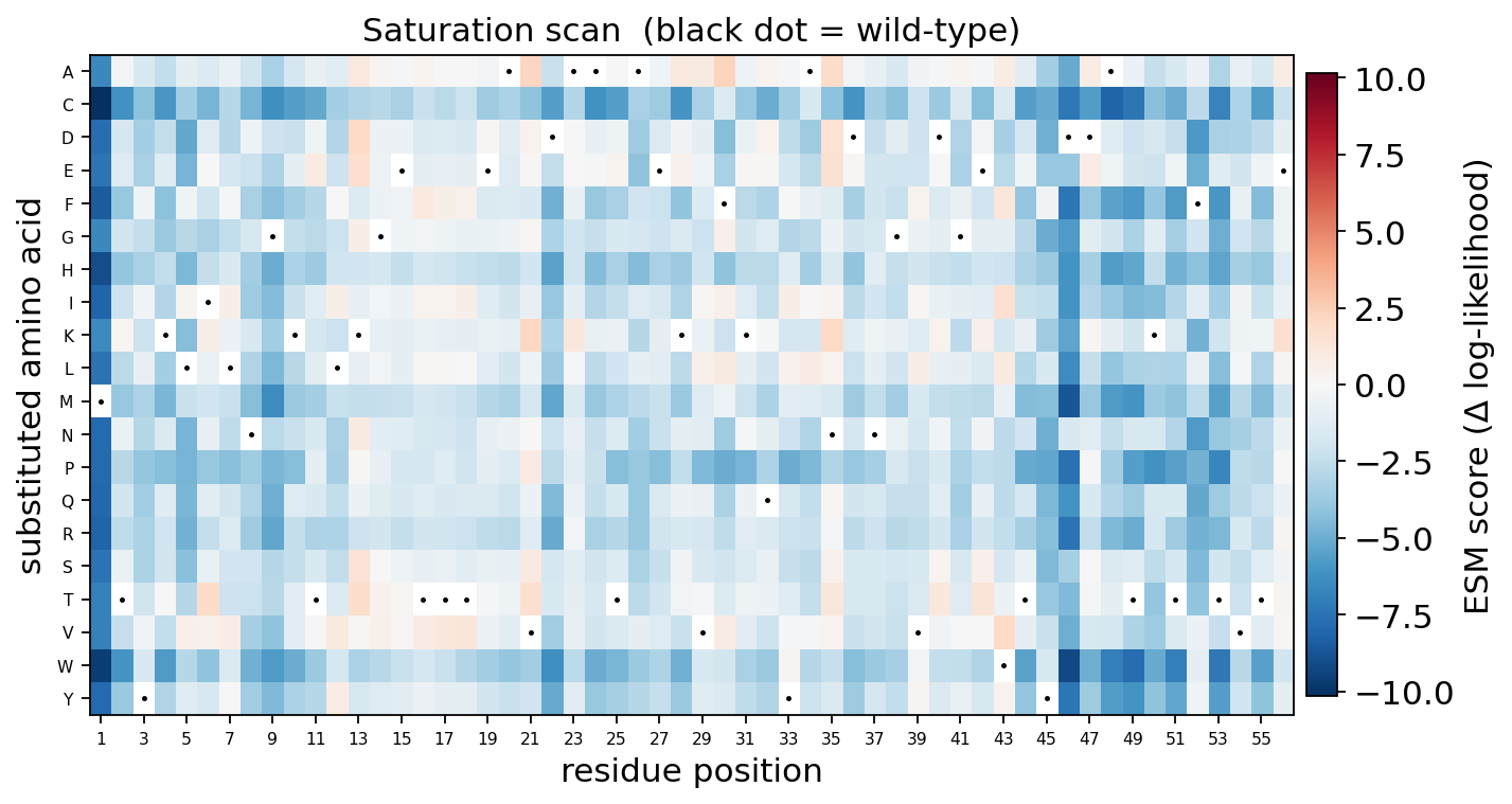
Rather than screen blindly, let a protein language model prioritise. ml_guided_design scores every single mutation with an ESM saturation scan, then greedily combines the most-favoured, non-conflicting mutations into ranked multi-mutant designs — a first-round design an experimentalist can order.

designs = ov.synbio.ml_guided_design(GB1, n_mutations=3, n_designs=6)
for d in designs[:4]:
    print('+'.join(d.mutations), ' predicted score', round(d.predicted_score, 2))
# protein logo over the designed variants — where directed evolution concentrates its edits
ov.synbio.plot_sequence_logo([d.sequence for d in designs], title='ML-guided GB1 variant library')
None

F30A+V21A+W43V  predicted score 6.49
F30A+V21A  predicted score 4.45
F30A  predicted score 2.28
F30A  predicted score 2.28

The design is built from the single-mutation landscape — the same ESM saturation scan, shown as a heatmap. Red cells are favoured substitutions; the greedy designer picks the best non-conflicting ones.

dms = ov.synbio.variant_effect(GB1, model='esm1v')
ov.synbio.plot_variant_effect(dms)
None

[ov.synbio.variant_effect] model=esm1v scoring=masked-marginals device=cuda (NVIDIA H100 80GB HBM3, 79 GB)

6 — Confirm the enzyme’s function (CLEAN)

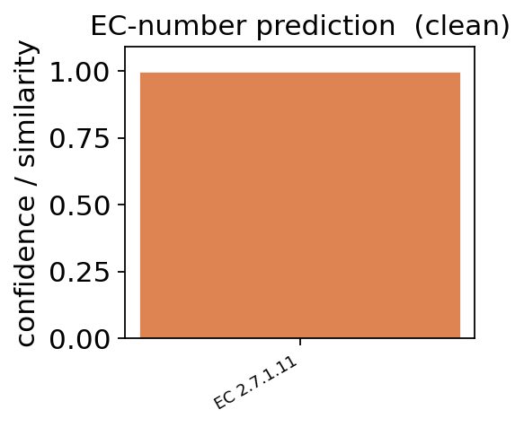
Before evolving an enzyme it helps to confirm what it does. enzyme_function predicts the EC number two ways: method='knn' (a light ESM-2 nearest-neighbour vs a small bundled reference) and method='clean' — the real trained CLEAN model (Yu 2023, contrastive ESM-1b assigned by max-separation against ~5,200 SwissProt EC cluster centres). On the real E. coli phosphofructokinase (PfkA), CLEAN returns the correct EC 2.7.1.11 with high confidence. plot_ec_prediction shows the ranked calls.

PFKA = ('MIKKIGVLTSGGDAPGMNAAIRGVVRSALTEGLEVMGIYDGYLGLYEDRMVQLDRYSVSDMINRGGTFLGSARFPEFRD'
        'ENIRAVAIENLKKRGIDALVVIGGDGSYMGAMRLTEMGFPCIGLPGTIDNDIKGTDYTIGFFTALSTVVEAIDRLRDT')
# baseline: ESM-2 k-NN vs a small bundled reference
knn = ov.synbio.enzyme_function(PFKA, method='knn', verbose=False)
# real SOTA: the trained CLEAN model (contrastive ESM-1b vs ~5,200 EC centres)
clean = ov.synbio.enzyme_function(PFKA, method='clean', verbose=False)
print('k-NN baseline :', knn.predictions[:2])
print('CLEAN (real)  :', clean.predictions[:2], '  true EC of PfkA = 2.7.1.11')
ov.synbio.plot_ec_prediction(clean)
None

k-NN baseline : [('2.7.1.11', 0.9837279915809631), ('4.2.1.11', 0.9466314315795898)]
CLEAN (real)  : [('2.7.1.11', 0.9912)]   true EC of PfkA = 2.7.1.11

Summary

From one protein we designed and scored CRISPR guides (with specificity screening and edit planning) and a directed-evolution campaign (libraries + model-guided variant selection) — the build and test/learn arms of the DBTL cycle, entirely inside ov.synbio.

Combine with the core tutorial (metabolism ↔ protein ↔ DNA) and tutorial II (circuits, assembly, pathway design) for the full picture.